In part 1, we extracted the games and ratings data via webscraping and api calls to the Boardgamegeek website.
In this section, we will be attempting to put these ratings through various models in order to generate recommendations for users on the website.
To recap, we have 120,679 users and 1807 games forming a N x M matrix of 120,679 x 1807 with a total of 7.7 million ratings. I have only selected users that have rated at least 10 games or more. Our matrix density is 3.54% or 96.45% sparse.
I will be utilizing both neighbourhood and latent factor models from the collaborative filtering approach to predict ratings for each user on the games he/she has yet to rate.
For the neighbourhood method, I will be employing the use of the cosine similarity function. As for the latent factor models, matrix factorization will be accomplished via the SVD method as well as non-negative matrix factorization method utilizing alternating least squares to optimize the loss function.
Offline evaluations will be conducted using RMSE.
The Approach and Setup
In general, here’s what we will be performing in order with each modeling technique:
- Acquire train and test sets
- Normalize train set ratings
- Fit train set on model instance
- Make predictions on test set
- Determine RMSE
- Provide recommendations for specified user
First we get our regular imports in along with some additional ones:
import pandas as pd
import numpy as np
import matplotlib.pyplot as plt
import seaborn as sns
import pickle
import sqlite3
from scipy import sparse
from sklearn.metrics import mean_squared_error

%config InlineBackend.figure_format = 'retina'
%matplotlib inline

sns.set_style('white')
We import scipy.sparse so that we can perform sparse matrix calculations on our sparse ratings matrix which speeds up calculations. The sparse format stores only the necessary data in 3 arrays and ignores all the other empty cells.
We also import mean_squared_error to aid us in our calculation of the Root Mean Squared Error(RMSE) evaluation metric.
df = pd.read_pickle('ratings_pickle')
df.shape
(120679, 1807)
We also import our pickled file from the part 1 and make sure it contains the matrix in the right shape
games = pd.read_csv('bgg_gamelist.csv')
Let’s not forget our gameslist as well which we will need to link with our ratings matrix through the gameids to identify the games recommended.
Creating the base class
I decided to create a base Recommender class so that I am able to reuse some of the basic preprocessing methods with other modeling techniques down the pipeline. It helps to organize the code neatly too.
The Recommender class contains methods for preprocessing the data before modeling. The class takes in a ratings dataframe and allows one to create a sparse representation of it, train-test split it, normalize the training set, calculate mean by users and overall mean as well as obtaining the RMSE score for model evaluation.
class Recommender(object):
    '''
    A class for building a recommender model

    Params
    ======
    ratings : (Dataframe)
        User x Item matrix with corresponding ratings

    '''

    def __init__(self, ratings):
        self.ratings = ratings

    def create_sparse(self, ratings):
        '''
        Creates sparse matrices by filling NaNs
        with zeros first
        '''
        ratings_sparse = sparse.csr_matrix(ratings.fillna(0))
        return ratings_sparse

    def train_test_split(self, ratings_sparse, test_size='default', train_size=None, random_state=None):
        '''
        Splits ratings data into train and test sets.
        This implementation ensures that each test set
        will have at least one rating from each user.

        Params
        ======
        ratings_sparse : (Sparse matrix)
            A sparse representation of the original matrix

        test_size : (int)
            An integer indicating number of random ratings
            from each user to be allocated to the test set

        train_size : (int)
            An integer indicating number of random ratings
            from each user to be allocated to the train set

        random_state : (int)
            Random seed for reproducibility
        '''
        r = np.random.RandomState(random_state)

        if test_size == 'default':
            test_size = None
        if test_size is None and train_size is None:
            test_size = 1
        if test_size == float or train_size == float:
            raise ValueError('test_size or train_size must be a positive integer')
        if train_size is not None:
            test_size = None

        if test_size is not None:
            train_set = self.ratings.copy().as_matrix()
            test_set = np.full(self.ratings.shape, np.nan)

            for idx, row in enumerate(ratings_sparse):
                #Get column ids based on random choice of available games in current user
                test_indices = r.choice(row.indices, test_size, replace=False)
                test_data = []
                for val in test_indices:
                    index = list(row.indices).index(val)
                    test_data.append(row.data[index])
                train_set[idx, test_indices] = np.nan
                test_set[idx, test_indices] = test_data
            train_set = pd.DataFrame(train_set, index=self.ratings.index, columns=self.ratings.columns)
            test_set = pd.DataFrame(test_set, index=self.ratings.index, columns=self.ratings.columns)

        else:
            test_set = self.ratings.as_matrix()
            train_set = np.full(self.ratings.shape, np.nan)

            for idx, row in enumerate(ratings_sparse):
                train_indices = r.choice(row.indices, train_size, replace=False)
                train_data = []
                for val in train_indices:
                    index = list(row.indices).index(val)
                    train_data.append(row.data[index])
                test_set[idx, train_indices] = np.nan
                train_set[idx, train_indices] = train_data
            train_set = pd.DataFrame(train_set, index=self.ratings.index, columns=self.ratings.columns)
            test_set = pd.DataFrame(test_set, index=self.ratings.index, columns=self.ratings.columns)

        assert self.ratings.notnull().sum().sum() == train_set.notnull().sum().sum() + test_set.notnull().sum().sum()

        return train_set, test_set


    def normalize(self, ratings_sparse):
        '''Normalizes each user by their mean. Accepts a sparse array'''
        ratings = np.zeros_like(self.ratings)
        for idx, i in enumerate(ratings_sparse):
            ratings[idx, i.indices] = i.data-i.data.mean()
        return ratings

    def get_user_mean(self):
        '''Calculate mean rating values for each user'''
        mean = np.mean(self.ratings, axis=1)
        return mean

    def get_overall_mean(self, mean):
        '''
        Outputs mean of entire dataframe

        Params
        ======

        mean : (pd.Series or nd_array)
            Vector of user means across their ratings
        '''
        mean_all = np.mean(mean)
        return mean_all

    def get_baseline_rmse(self, test, mean_all):
        '''
        Ouputs the baseline rmse by comparing test
        set ratings with the mean rating for each user

        Params
        ======

        test : (nd_array)
            Numpy array of test results

        test_sparse : (Sparse matrix)
            Sparse representation of test matrix

        mean_all : (float)
            Value of mean of entire ratings matrix
        '''
        actual = test[test.nonzero()].flatten()
        preds = [mean_all for val in test[test.nonzero()].flatten()]
        prediction = preds
        return np.sqrt(mean_squared_error(actual, prediction))

    def get_rmse(self, test, prediction):
        '''
        Returns the rmse score from a prediction result

        Params
        ======

        test : (nd_array
            Numpy array of test results

        prediction (nd_array)
            Predicted scores after training through model
        '''
        actual = test[test.nonzero()].flatten()
        prediction = prediction[prediction.nonzero()].flatten()
        return np.sqrt(mean_squared_error(actual, prediction))
The most interesting method in the base class would probably be the train_test_split method as I had to create one to ensure that a certain number of ratings would be in the test set for each user as opposed to a random assignment. In my implementation, you are able to enter the number of ratings you want in the test set or the training set. It is possible to set a low training set value to simulate the cold start problem using this function.
Neighbourhood method - Cosine similarity recommender
Our first method to determine recommendations is by calculating the similarity between users and items. I have decided to employ the cosine similarity function owing to its favourable representation in the recommender systems community.
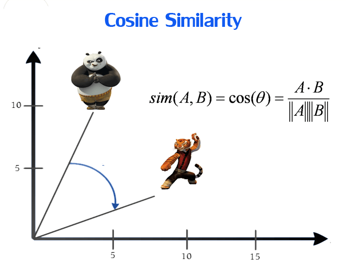 The cosine similarity function measures the cosine angle between 2 vectors, and in our case, between 2 game or user vectors of our ratings matrix. It is calculated by the dot product of the vectors over the magnitude of each vector. It outputs the cosine similarity score to evaluate how similar 2 vectors are to each other.
A similarity matrix is first obtained between each item pair or user pair. A prediction function is then used to predict ratings for results held out in the test set in order to compare the accuracy through the RMSE loss function.
In this case, we will only be utilizing item-item similarities as our neighborhood method of choice due to less intensive computation required.
A subclass was built off the base Recommender class so as to be able to utilize some of its functions like calculating RMSE which will be used for all our models.
from sklearn.metrics.pairwise import cosine_similarity

class CosineSim(Recommender):
    '''
    A Recommender class that uses the cosine similarity
    function to recommend games

    Params
    ======
    ratings : (Dataframe)
        Ratings matrix
    '''
    def __init__(self, ratings):
        self.ratings = ratings

    def find_similarity(self, ratings_sparse, kind='item'):
        '''
        Finds the cosine similarity in either
        item-item or user-user configurations
        of a sparse matrix

        Params
        ======
        ratings_sparse : (Sparse matrix)
            Sparse representation of ratings matrix

        kind : (string)
            Default is item for item-item similarity.
            Other option is user for user-user similarity
        '''
        if kind == 'item':
            similarities = cosine_similarity(ratings_sparse.T)
        elif kind == 'user':
            similarities = cosine_similarity(ratings_sparse)
        return similarities

    def predict_for_test(self, train, test_sparse, similarity, kind='item'):
        '''
        Predicts the scores for games in test set

        Params
        ======
        train : (Dataframe)
            Dataframe of training set

        test_sparse : (Sparse matrix)
            Sparse representation of test set

        similarity : (nd_array)
            Similarity matrix of user-user or item-item pairs

        kind : (string)
            Default is 'item' for item-item predictions.
            Alternative is 'user' for user-user predictions

        '''
        prediction = np.zeros_like(train)

        if kind == 'item':
            train = train.fillna(0).as_matrix()
            for row, val in enumerate(test_sparse):
                for col in val.indices:
                    sim = similarity[col]
                    rated = train[row].nonzero()
                    prediction[row, col] = np.sum(sim[rated]*train[row][rated])/np.sum(np.abs(sim[rated]))

        elif kind == 'user':
            mean  = train.apply(np.mean, axis=1)
            std = train.apply(np.std, axis=1)

            for row, val in enumerate(test_sparse):
                avg_rating = mean.iloc[row]
                sim = similarity[row]
                ind_std = std.iloc[row]

                for col in val.indices:
                    prediction[row, col] = avg_rating + np.sum(sim*train.iloc[:, col])/np.sum(np.abs(sim))

        return prediction

    def recommend(self, user, similarity, games, kind='item'):
        '''
        Recommends list of games to specified user

        Params
        ======
        user : (string)
            username with at least 10 ratings in database

        similarity : (nd_array)
            Similarity matrix of user-user or item-item pairs

        games : (Dataframe)
            Dataframe of game list

        kind : ('string)
            Default is 'item' for item-item predictions.
            Alternative is 'user' for user-user predictions
        '''
        preds = np.zeros_like(self.ratings.loc[user])

        if kind == 'item':
            ratings_array = self.ratings.fillna(0).as_matrix()
            person = ratings_array[self.ratings.index.get_loc(user)]
            rated = person.nonzero()[0]
            for idx in range(ratings_array.shape[1]):
                if idx not in rated:
                    sim = similarity[idx]
                    preds[idx] = np.sum(sim[rated]*person[rated])/np.sum(np.abs(sim[rated]))

        elif kind == 'user':

            rated = self.ratings.loc[user].dropna().index
            std = np.std(self.ratings.loc[user])
            mean  = np.mean(self.ratings.loc[user])
            sim = similarity[self.ratings.index.get_loc(user)]

            for idx, col in enumerate(ratings.columns):
                if col not in rated:
                    preds[idx] = mean + np.sum((sim*ratings[col]))/np.sum(np.abs(sim))

        predictions = pd.Series(preds, index=self.ratings.columns, name='predictions')
        recommendations = games.join(predictions, on='gameid')
        return recommendations.sort_values('predictions', ascending=False)
I have allocated the ability to select user-user or item-item calculations for the find_similarity, predict_for_test and recommend functions which works on a smaller toy dataset. It would be interesting to note that the prediction function I coded for this Cosine Similarity model predicts only for the holdout values on the test set and not on the entire matrix for the sake of computational speed.
Following our general approach, here are the steps to model, predict and generate recommendations utilizing the Cosine Similarity function:
Preprocess data
#Creating an instance of the Recommnder class
rec = Recommender(df)

#Creating a sparse matrix of the full data
df_sparse = rec.create_sparse(df)

#Performing train-test split
%time train, test = rec.train_test_split(df_sparse, test_size=2, random_state=123)

#Create sparse matrix for training set
train_sparse = rec.create_sparse(train)

#Create sparse matrix for test set
test_sparse = rec.create_sparse(test)
We split the matrix such that there are 2 ratings in the test set for each user. I chose the value of 2 so that for our raters with only 10 ratings, I have at least 80% of their ratings data to predict on their remaining 20%.
Modeling - Create Similarity Matrix
#Create an instance of the Cosine Similarity Recommender class
cossim = CosineSim(df)
The first thing we should normally do is normalize the training set to account for variances in how users rate the games. We do not normalize the training set here as the cosine similarity function from sklearn already does it for us.
#Acquiring item-item similarity matrix
%time item_sims = cossim.find_similarity(train_sparse)

CPU times: user 5.83 s, sys: 357 ms, total: 6.19 s
Wall time: 6.3 s
Predicting scores on test set
#Predicting the scores for test set
%time item_preds = cossim.predict_for_test(train, test_sparse, item_sims)

CPU times: user 36 s, sys: 5.92 s, total: 41.9 s
Wall time: 43.5 s
We measure wall time so we can appreciate how long it takes to generate these recommendations which is important when we decide to push it to production.
Evaluate with RMSE
First we calculate our baseline RMSE which is taken as the same value of the mean rating for the entire dataset predicted for each datapoint in the test set.
#Converting test set to an array
y = test.fillna(0).values

#Getting user means
mean = rec.get_user_mean()

#Calculating overall mean
overall_mean = rec.get_overall_mean(mean)
overall_mean

7.398810764577983

#Computing baseline error
baseline_error = rec.get_baseline_rmse(y, overall_mean)
baseline_error

1.4869803145678728
We then calculate our RMSE score for the Cosine Similarity model.
#Calculating the error
error_cos = cossim.get_rmse(y, item_preds)
error_cos

1.3339479358142938
We can observe a decrease of about 10% from the baseline score.
Performing recommendations
We will be performing recommendations for myself as I am an active user of the site and have rated quite a number of games (226 to be exact). We calculate the similarity matrix again, this time utilizing the entire dataset before making the predictions and utilizing the recommendation function
#Calculate item-item similarity matrix of entire ratings data
%time all_sims = cossim.find_similarity(df_sparse)
CPU times: user 5.9 s, sys: 359 ms, total: 6.26 s
Wall time: 6.4 s
#Perform recommendation for a specific user
%time me_cos = cossim.recommend('passthedynamite', all_sims, games)
CPU times: user 10 s, sys: 5.39 s, total: 15.4 s
Wall time: 16.6 s
#Observe top 20 recommendations
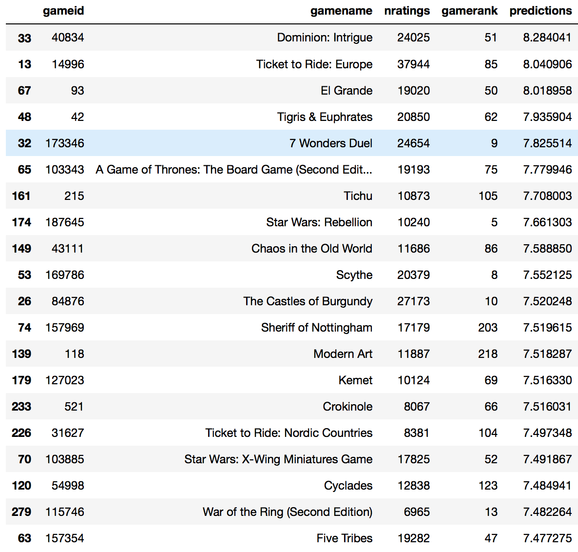
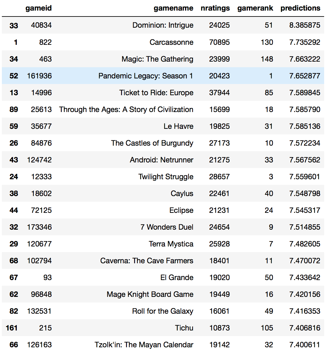
me_cos.head(20)
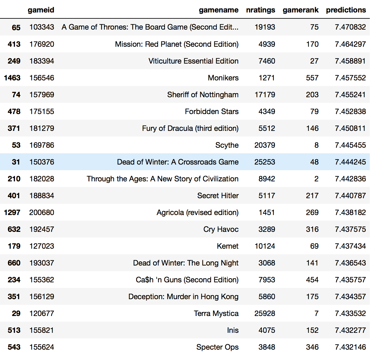 An example of how a top 20 list would look like
This list of games is quite an interesting one. I own one of the games (Cry Havoc) and have yet to play it but purchased it after performing intensive research. Several of the games like Dead of Winter, Viticulture and Scythe are in my wishlist. There are some games that I have looked at but have no interest in trying like Cash n Guns and Forbidden Stars. Most of the other games I am aware of but have not done deeper research which suggests that I should do so based on its recommendation. One thing interesting about this list is the range of games it provides. It does not include solely the top games as determined by the game rank but has a good mix from the top 600. In fact, Monikers, ranked 557, is one I have never heard of till now.
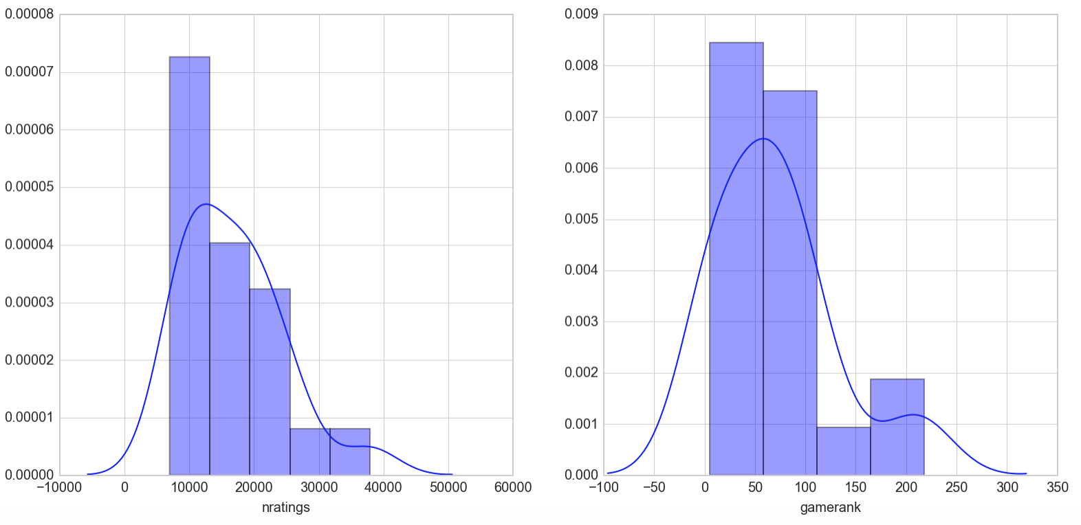
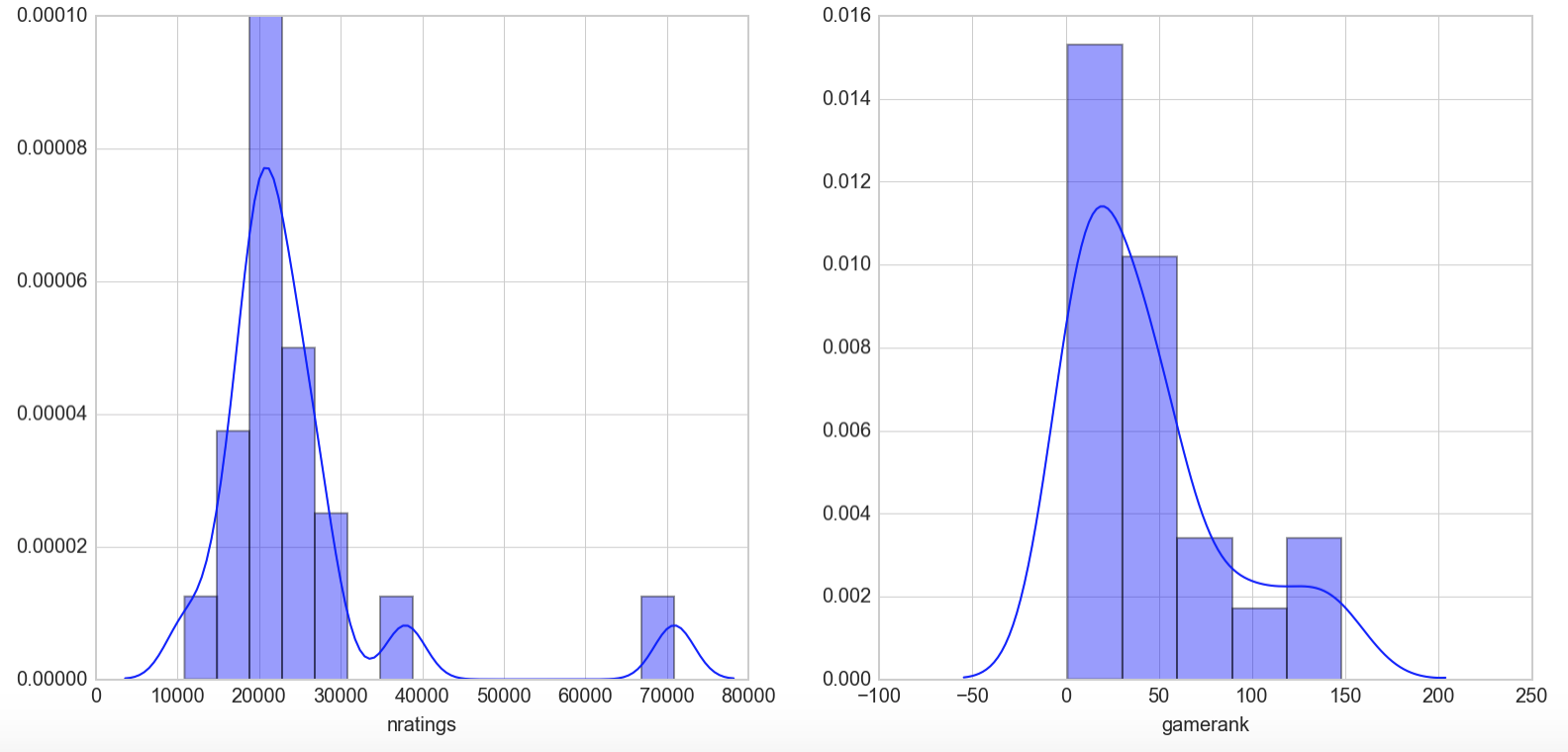
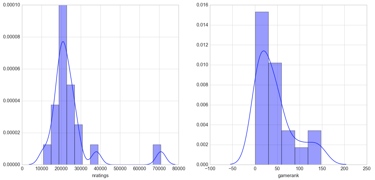
Let’s take a look at the distribution of this list of 20 games in terms of number of ratings and ranking on Boardgamegeek.
As an interesting tidbit, Games are ranked on BGG based on a value called the Geek rating which is essentially a bayesian average of all the ratings a game receives. The prior mean, thought to be 5.5, is multiplied by a constant, C, and is factored into the calculation of a game’s average rating. This is done to prevent new games from being manipulated into entering the ranking system at a high level with just a few ratings. C is unknown but is thought to be 100.
fig, ax = plt.subplots(1,2, figsize=(13,6))
sns.distplot(me_cos.head(20)['nratings'], ax=ax[0])
sns.distplot(me_cos.head(20)['gamerank'], ax=ax[1])
plt.show()
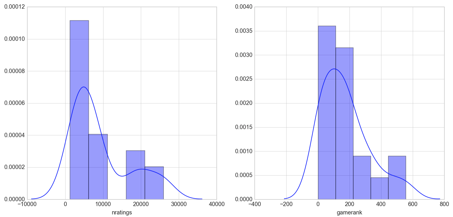
Most of the games in this top 20 list have less than 5000 ratings which seems to suggest a rather good spread of game popularity in its recommendation. For reference, the maximum number of ratings for a game in our dataset is 71,279 and the least is 975.
The majority of the games recommended also lies between 1-200 in gamerank which suggests that the recommender is recommending me games that have a high approval rate with the user population. The spread is not too bad hitting games that rank in the 500s. This is more diverse than some lists recommended further down as we shall soon see. For reference, the top ranked game in our database is 1 while the least is 14344
Latent factor method - Singular Value Decomposition
The latent factor method decomposes the sparse ratings matrix into a set of latent vectors for both users and items. These are low rank approximations of the original matrix and helps to address the issue of sparsity that is characteristic of any form of explicit rating data.
It should be understood that the latent space that is created by mapping both user and items onto is made up of item and user features, some of which are explainable like theme and mechanics of the game, a user’s preference for certain genres and game difficulties to unexplainable concepts. Each user and item can be explained by some combination of these factors and therefore predictions of a user’s preference for an item can be made through a simple dot product of the user’s latent vector by the transpose of that item’s corresponding latent vector.
We explore this concept with the Singular Value Decomposition of the ratings matrix first.
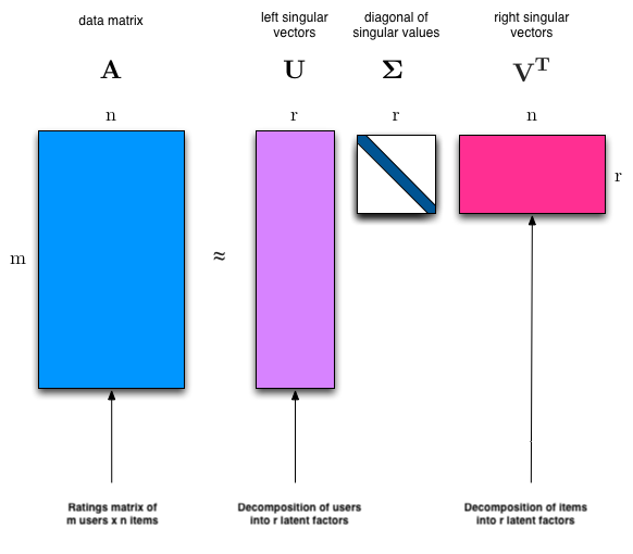 A sparse User-Item matrix is decomposed(broken down) into 3 components: A user matrix explained by r latent factors, an item matrix explained by r latent factors and a matrix that contains the non-negative singular values in descending order along the its diagonal. The singular values determine the magnitude of effect of the latent factors in determining the predictions. A dot product of the 3 matrices solves for the larger matrix it was decomposed from.
We build a subclass from our base Recommender class to represent the SVD model. In it, we will be using the svds function of the scipy sparse library that takes in a sparse matrix and finds the largest k singular values of the matrix where k is the number of latent factors specified.
from scipy.sparse.linalg import svds
class SVD(Recommender):
    '''
    A model for getting game recommendations by
    calculating singular values through matrix
    decomposition into its latent factors

    Params
    ======
    ratings : (nd_array)
        Normalized ratings array
    '''
    def __init__(self, normed_ratings):
        self.normed_ratings = normed_ratings

    def train(self, k=50):
        '''
        Trains SVD model on ratings

        Params
        ======
        k : (int)
            Specifies number of latent factors to decompose into
        '''
        U, sigma, Vt = svds(self.normed_ratings, k)
        sigma = np.diag(sigma)
        return U, sigma, Vt

    def predict(self, U, sigma, Vt, test, mean):
        '''
        Outputs predictions for entire ratings matrix as well
        as for test set.

        Params
        ======
        test : (Dataframe)
            Test set pandas dataframe

        mean : (pd.Series)
            Vector of user means
        '''
        all_predictions = np.dot(np.dot(U, sigma), Vt) + mean.reshape(-1, 1)
        test_predictions = all_predictions[test.fillna(0).as_matrix().nonzero()]

        return all_predictions, test_predictions

    def recommend(self, ratings, user, games, predictions):
        '''
        Provides recommendations for the specified user

        Params
        ======
        user : (string)
            username with at least 10 ratings in database

        games : (Dataframe)
            Dataframe of game list

        predictions : (nd_array)
            predictions of entire ratings matrix
        '''
        user_idx = ratings.index.get_loc(user)
        preds = predictions[user_idx]
        rated = ratings.loc[user].fillna(0).as_matrix().nonzero()

        mask = np.ones_like(preds, dtype=bool)
        mask[rated] = False
        preds[~mask] = 0

        predictions = pd.Series(preds, index=ratings.columns, name='predictions')
        recommendations = games.join(predictions, on='gameid')
        return recommendations.sort_values('predictions', ascending=False)
Unlike the cosine similarity class, our the prediction function in our SVD class predicts for the entire matrix and not just the test set. Because of this, our recommend function needs to be tweaked from that of the cosine similarity class.
Normalize, instantiate and train
 #Normalize training set
train_normed = rec.normalize(train_sparse)

#Instatiate SVD class
svd_train = SVD(train_normed)

#Train SVD model
%time U, sigma, Vt = svd_train.train(k=50)

CPU times: user 1min 33s, sys: 1.25 s, total: 1min 34s
Wall time: 49.5 s
We start off by training an SVD model with 50 latent factors
Obtain predictions for test set and evaluate RMSE
#Make predictions for test set
%time all_preds_svd50_train, test_preds_svd50 = svd_train.predict(U, sigma, Vt, test, mean)

#Evaluate RMSE for k=50
error_svd50 = svd_train.get_rmse(y, test_preds_svd50)
error_svd50

1.2861092502817428
This value is 3% less than the value calculated for the Cosine Similarity method.
Recommend games
In performing recommendations, we utilize the entire dataset, not just the train set, so as to provide the most accurate and relevant suggestions.
#Recommend games for a specific user
%time me_svd_50 = svd.recommend(df, 'passthedynamite', games, all_preds_svd50)
#Displaying top 20 games with k=50
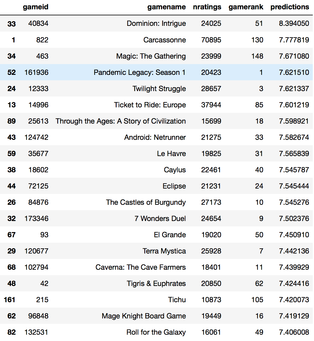
me_svd_50.head(20)
This list of games seem to be restricted to games within the top 200 or so. As it is, I am aware of all the games and have variations of some of the games listed such as Ticket to Ride: Europe and Dominion: Intrigue. I actually rate their sister games really highly which is why they appear.
While the maximum number of ratings was in the 20,000s for the cosine similarity model, the SVD model is giving me games that hit the high 30,000s in number of ratings. A look at the gamerank distribution also shows that the games fall between ranks 1-200 which suggests less diversity from the top-ranked games.
What if we were to change the number of latent factors to 100?
#Train SVD model with k=100
%time U, sigma, Vt = svd_train.train(k=100)

#Make predictions
%time all_preds_svd100_train, test_preds_svd100 = svd_train.predict(U, sigma, Vt, test, mean)

#Evaluate RMSE for k=100
error_svd_100 = svd_train.get_rmse(y, test_preds_svd100)
error_svd_100

1.2954613798828805
The result is slightly worse than k=50 but still remains better than the RMSE for cosine similarity
#Recommend games for a specific user
%time me_svd_100 = svd.recommend(df, 'passthedynamite', games, all_preds_svd100)

#Displaying top 20 games with k=100
me_svd_100.head(20)
Most of the games recommended come from the top 100 games. One big surprise here is that tic-tac-toe was actually recommended. A quick check reveals that it is the bottom-ranked game from the 1807 in our dataset. The list is really different from the previous 2 but nothing I have not seen or heard before. Not much serendipity here.
The lower end of number of ratings of games in this list seems to have shifted up with the majority being at the 10,000s range. We can also see the outlier of the last-ranked game of our list that severely skews our gamerank distribution.
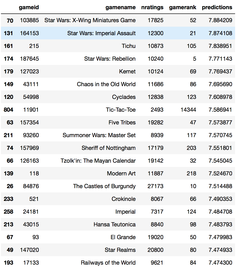
Let’s go the other way and train on 10 latent factors
#Train SVD model with k=10
%time U, sigma, Vt = svd_train.train(k=10)

#Make predictions
%time all_preds_svd10_train, test_preds_svd10 = svd_train.predict(U, sigma, Vt, test, mean)

#Evaluate RMSE for k=10
error_svd_10 = svd_train.get_rmse(y, test_preds_svd10)
error_svd_10

1.2784756733580973
With 10 latent factors, I get my lowest RMSE score yet. Let’s see what games it recommends to me.
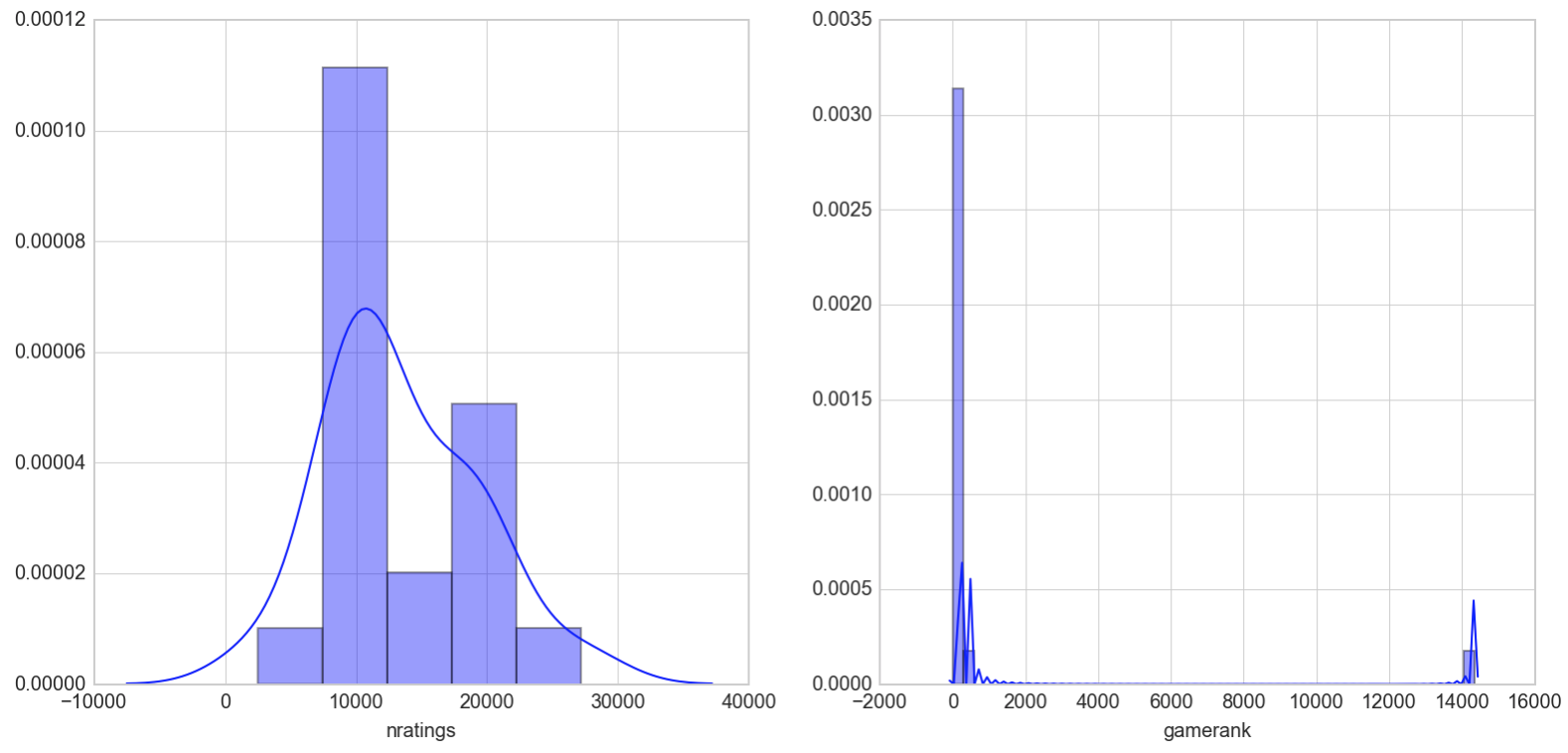
The majority of these games are within the top 100 games which suggests that they are highly popular and well-regarded. I am intersted in trying some of these games but don’t like the number 2 game of which I had previously rated a similar version quite poorly. Let’s take a look at the distributions of the number of ratings and gamerank
As suspected, this list contains the top regarded games on BGG. This can be observd through the smaller range of games recommended in terms of gamerank from 1-150 and the inclusion of a game with a high number of ratings, Carcassone with 70895 ratings to be exact. The lower end of the number of ratings has also shifted to games where at least 10,000 users have rated the game.
Latent Factor model - Non-Negative Matrix Factorization with Alternating Least Squares
In this final model, we will attempt to factorize the ratings matrix using the Alternating Least Squares method of optimizing the cost function. It works by holding one set of latent factors, either the user or item vector, constant at any one point in time while solving a linear equation for the other. It then alternates until convergence to a minimum. As opposed to SVD, bias terms are added to the cost function and singular values are not calculated.
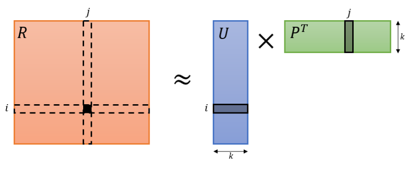 R is the ratings matrix, U is the user matrix bounded by k latent factors and P is a transposed item matrix bounded by k latent factors. For a user i on item j, solving for Rij is simply a dot product of the Uik vector and the PTik vector.
The cost function for matrix factorization depicted below is represented as solving for the mean squared error of the original rating matrix R with its approximation U x PT as its first term and with regularization terms accounting for user and item biases in its second term.

A class is built off the base Recommender class and a grid search was applied to find the best hyperparameters of regularization, number of iterations of the alternating least squares step as well as the optimal number of latent factors.
from numpy.linalg import solve
class ALSMF(Recommender):
    def __init__(self,
                 ratings,
                 n_factors=40,
                 item_reg=0.0,
                 user_reg=0.0,
                 verbose=False):
        """
        Train a matrix factorization model to predict empty
        entries in a matrix. The terminology assumes a
        ratings matrix which is ~ user x item

        Params
        ======
        ratings : (ndarray)
            User x Item matrix with corresponding ratings

        n_factors : (int)
            Number of latent factors to use in matrix
            factorization model

        item_reg : (float)
            Regularization term for item latent factors

        user_reg : (float)
            Regularization term for user latent factors

        verbose : (bool)
            Whether or not to printout training progress
        """
        self.ratings = ratings
        self.n_users, self.n_items = ratings.shape
        self.n_factors = n_factors
        self.item_reg = item_reg
        self.user_reg = user_reg
        self._v = verbose

    def als_step(self, latent_vectors, fixed_vecs, ratings, _lambda, type='user'):
        """
        One of the two ALS steps. Solve for the latent vectors
        specified by type.
        """
        if type == 'user':
            # Precompute
            YTY = fixed_vecs.T.dot(fixed_vecs)
            lambdaI = np.eye(YTY.shape[0]) * _lambda

            for u in xrange(latent_vectors.shape[0]):
                latent_vectors[u, :] = solve((YTY + lambdaI),
                                             ratings[u, :].dot(fixed_vecs))
        elif type == 'item':
            # Precompute
            XTX = fixed_vecs.T.dot(fixed_vecs)
            lambdaI = np.eye(XTX.shape[0]) * _lambda

            for i in xrange(latent_vectors.shape[0]):
                latent_vectors[i, :] = solve((XTX + lambdaI),
                                             ratings[:, i].T.dot(fixed_vecs))
        return latent_vectors

    def train(self, n_iter=10):
        """ Train model for n_iter iterations from scratch."""
        # initialize latent vectors
        self.user_vecs = np.random.random((self.n_users, self.n_factors))
        self.item_vecs = np.random.random((self.n_items, self.n_factors))

        self.partial_train(n_iter)

    def partial_train(self, n_iter):
        """
        Train model for n_iter iterations. Can be
        called multiple times for further training.
        """
        ctr = 1
        while ctr <= n_iter:
            if ctr % 10 == 0 and self._v:
                print '\tcurrent iteration: {}'.format(ctr)
            self.user_vecs = self.als_step(self.user_vecs,
                                           self.item_vecs,
                                           self.ratings,
                                           self.user_reg,
                                           type='user')
            self.item_vecs = self.als_step(self.item_vecs,
                                           self.user_vecs,
                                           self.ratings,
                                           self.item_reg,
                                           type='item')
            ctr += 1

    def predict(self, test, mean):
        """
        Predicts ratings based on user and
        item latent factors
        """
        all_predictions = self.user_vecs.dot(self.item_vecs.T) + mean.reshape(-1, 1)
        test_predictions = all_predictions[test.fillna(0).as_matrix().nonzero()]
        return all_predictions, test_predictions

    def recommend(self, ratings, user, games, predictions):
        '''
        Provides recommendations for the specified user

        Params
        ======
        user : (string)
            username with at least 10 ratings in database

        games : (Dataframe)
            Dataframe of game list

        predictions : (nd_array)
            predictions of entire ratings matrix
        '''
        user_idx = ratings.index.get_loc(user)
        preds = predictions[user_idx]
        rated = ratings.loc[user].fillna(0).as_matrix().nonzero()

        mask = np.ones_like(preds, dtype=bool)
        mask[rated] = False
        preds[~mask] = 0

        predictions = pd.Series(preds, index=ratings.columns, name='predictions')
        recommendations = games.join(predictions, on='gameid')
        return recommendations.sort_values('predictions', ascending=False)
The predict and recommend methods are the same as that for the SVD class. The only difference being in how the train method is constructed with the ALS step function used to solve for the latent vectors.
Here’s the implementation of the grid search algorithm. I limited it to no more than 20 latent factors and 40 iterations of the ALS step in the interest of time. (The entire process took about 5 hours!)
#Gridsearch of best parameters for ALS matrix factorization of ratings matrix
%%time
latent_factors = [5, 10, 20]
regularizations = [0.1, 1., 10., 100.]
regularizations.sort()
iter_array = [1, 10, 40]

best_params = {}
best_params['n_factors'] = latent_factors[0]
best_params['reg'] = regularizations[0]
best_params['n_iter'] = 0
best_params['test_rmse'] = np.inf
best_params['model'] = None

for fact in latent_factors:
    print 'Factors: {}'.format(fact)
    for reg in regularizations:
        print 'Regularization: {}'.format(reg)
        for itera in iter_array:
            print 'Iterations: {}'.format(itera)
            MF_ALS = ALSMF(train_normed, n_factors=fact, \
                                user_reg=reg, item_reg=reg)
            MF_ALS.train(n_iter = itera)
            all_predictions, test_predictions = MF_ALS.predict(test, mean)
            test_rmse = MF_ALS.get_rmse(y, test_predictions)
            if test_rmse < best_params['test_rmse']:
                best_params['n_factors'] = fact
                best_params['reg'] = reg
                best_params['n_iter'] = itera
                best_params['test_rmse'] = test_rmse
                best_params['model'] = MF_ALS
                print 'New optimal hyperparameters'
                print pd.Series(best_params)
The best parameters achieved were 40 iterations of the ALS step, of 10 factors with a regularization value of 0.1.
Train, predict, evaluate
Next we plug these values into an instance of the ALS class, predict the values and evaluate with RMSE.
#Instatiate ALSMF class
als_train = ALSMF(train_normed, n_factors=10, item_reg=0.1, user_reg=0.1)

#Train model
%time als_train.train(40)

#Make predictions for test set
%time all_preds_train, test_preds_train = als_train.predict(test, mean)

#Evaluate RMSE on test set
error_als = als_train.get_rmse(y, test_preds_train)
error_als

1.2785146629039117
The error looks to be almost as low as that generated by the SVD model with 10 latent factors. We will do a comparison below across the different models. Before that, let’s look at the recommendations generated by this model.
Much like the SVD model with 10 latent factors , the results for this list of 20 consists of games that are high in the board game geek rankings and looks very similar to that list.
The plots for the non-negative matrix factorization model looks just like that for SVD with 10 latent factors
Evaluating the models
So far, we have performed 2 types of offline evaluations. The RMSE scores for each model and a personal evaluation of the top 20 lists recommended to me through each algorithm. While the latter technique is less scientific, I believe it matters in the real world context as I consider myself a potential user of such a system and will evaluate its usefulness in recommending me items to explore and consider.
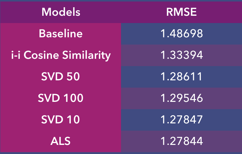
Through this table, we can observe that the models all performed better than baseline in minimizing RMSE. What’s surprising though is that the lower the number of latent factors, the better the model, but not by much. According to this set of results, it would seem that the SVD model with 10 latent factors performed the best while the cosine similarity model performed the worst.
As for comparison of the various top 20 lists generated, I liked most of the lists generated except the one with Tic Tac Toe recommended (SVD with 100 latent factors). I deduce that with that many latent factors, artificial meaning has to be ascribed to my relatively small sample size of 1807 games, such that it dilutes the importance of other key features, resulting in significant prediction error.
If I had to choose one list, I would go with the Cosine Similarity one as it contains the widest range of games with the most serendipituous recommendations.
Which model is best?
We have seen the results of the recommendations and the RMSE scores. Judging solely by the RMSE scores we are inclined to conclude that matrix factorization with 10 latent factors (SVD or NNMF) yields the most accurate scores. However, the top 20 lists they produce seem to only include games that are already popular on the website, which begs the question, what determines popularity of a game, the number of ratings or its rank?
#Plot scatterplot of number of ratings vs gamerank
sns.jointplot(games['nratings'], games['gamerank'])
plt.show()
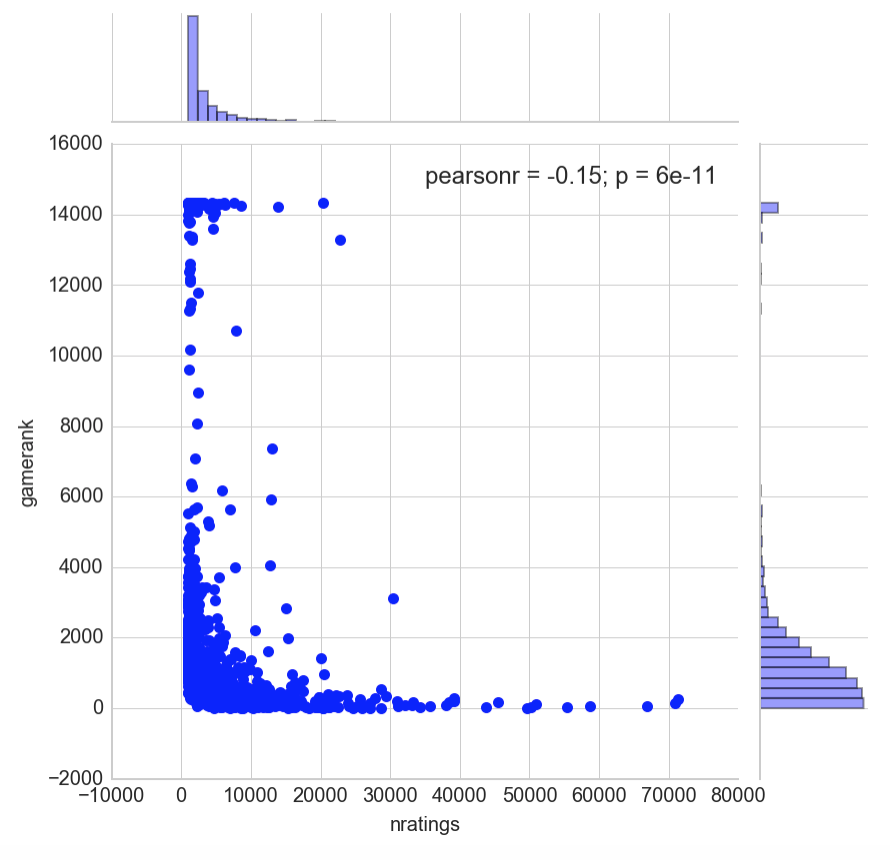
A quick look at the correlation between both variables suggests that there is little to no correlation between a game’s rank and how many users have rated it. Even so, we can observe that the most rated games tend to trend near the top of the rankings, while those at the bottom of the ranking chart generally receives fewer ratings.
Users that rate games on the site are quite a serious bunch and most likely would have looked for games via the ranking system first. The thing is, not all games on the top 100-200 will appeal to everyone and there is merit to recommending popular games that you will likely enjoy. However, the sense of serendipity is not there with lists that are too ‘rigid’ in their presentation. I was actually pleasantly surprised to discover a new game that was recommended to me via the ‘lesser’ cosine similarity algorithm.
The quality of a board game recommender system also depends on what it is positioned to accomplish. If it is to help one narrow down the choices of games to play or purchase next, it would seem that having high accuracy on the most popular games would help. On the other hand, if it is to discover new games on a regular basis, a less accurate but more serendipitous version would be ideal.
An ideal boardgame recommender system for BoardGameGeek users, at least to me personally, would be one that recommends me games from the popular bunch to look out for but also throws in some surprises with games that are further down the ranking order. Perhaps even 2 or more sets of top 20s with explanations such as “High-ranked games you might like’ and ‘Hidden gems similar to your taste’ etc.
Summary
In this second part of 3, I created python classes for my recommender system pipeline, took the ratings matrix and put it through 5 different models. These generated 5 sets of predictions that I then used to compare with the test set and evaluated them offline through RMSE scores. I also gave my personal take on the top 20 lists that were recommended for me.
Coming Up
In the next and final installment, we will be constructing our web app recommender system with Flask, deploy it on an Amazon EC2 instance and evaluate the results online to see which list out of three users of Boardgamegeek.com prefer.
This is part 2 of a 3 part series on building a board game recommender system for Boardgamegeek.com users. Part 1, where we scrape for ratings data can be found here. Part 3, where we build a web app and collect online evaluations can be found here.
The accompanying ipython notebook can be found in the following Github repo.