Everyone knows about the Boston Housing Dataset. But I bet you might not have heard of the Ames, Iowa Housing dataset. It was featured as part of a Kaggle competition 2 years back and was significant in how it tested advanced regression techniques in the form of creative feature engineering and feature selection.
In this 3 part series, I will be going through my approach to exploring the data in the first post, followed by linear regression modeling in order to predict housing prices based on features that are non-renovatable in the second. The 3rd and final part will bring in the renovatable features to identify what features offer the best value in improving the final selling price of the house.
Imports and Overview
We first perform the usual imports
import numpy as np
import scipy.stats as stats
import seaborn as sns
import matplotlib.pyplot as plt
import pandas as pd

sns.set_style('whitegrid')

%config InlineBackend.figure_format = 'retina'
%matplotlib inline
Next we load the data
house = pd.read_csv('./housing.csv')
You will want to refer to the data dictionary file to follow along with the description of the different features in our dataset.
house.info()
<class 'pandas.core.frame.DataFrame'>
RangeIndex: 1460 entries, 0 to 1459
Data columns (total 81 columns):
Id               1460 non-null int64
MSSubClass       1460 non-null int64
MSZoning         1460 non-null object
LotFrontage      1201 non-null float64
LotArea          1460 non-null int64
Street           1460 non-null object
Alley            91 non-null object
LotShape         1460 non-null object
LandContour      1460 non-null object
Utilities        1460 non-null object
LotConfig        1460 non-null object
LandSlope        1460 non-null object
Neighborhood     1460 non-null object
Condition1       1460 non-null object
Condition2       1460 non-null object
BldgType         1460 non-null object
HouseStyle       1460 non-null object
OverallQual      1460 non-null int64
OverallCond      1460 non-null int64
YearBuilt        1460 non-null int64
YearRemodAdd     1460 non-null int64
RoofStyle        1460 non-null object
RoofMatl         1460 non-null object
Exterior1st      1460 non-null object
Exterior2nd      1460 non-null object
MasVnrType       1452 non-null object
MasVnrArea       1452 non-null float64
ExterQual        1460 non-null object
ExterCond        1460 non-null object
Foundation       1460 non-null object
BsmtQual         1423 non-null object
BsmtCond         1423 non-null object
BsmtExposure     1422 non-null object
BsmtFinType1     1423 non-null object
BsmtFinSF1       1460 non-null int64
BsmtFinType2     1422 non-null object
BsmtFinSF2       1460 non-null int64
BsmtUnfSF        1460 non-null int64
TotalBsmtSF      1460 non-null int64
Heating          1460 non-null object
HeatingQC        1460 non-null object
CentralAir       1460 non-null object
Electrical       1459 non-null object
1stFlrSF         1460 non-null int64
2ndFlrSF         1460 non-null int64
LowQualFinSF     1460 non-null int64
GrLivArea        1460 non-null int64
BsmtFullBath     1460 non-null int64
BsmtHalfBath     1460 non-null int64
FullBath         1460 non-null int64
HalfBath         1460 non-null int64
BedroomAbvGr     1460 non-null int64
KitchenAbvGr     1460 non-null int64
KitchenQual      1460 non-null object
TotRmsAbvGrd     1460 non-null int64
Functional       1460 non-null object
Fireplaces       1460 non-null int64
FireplaceQu      770 non-null object
GarageType       1379 non-null object
GarageYrBlt      1379 non-null float64
GarageFinish     1379 non-null object
GarageCars       1460 non-null int64
GarageArea       1460 non-null int64
GarageQual       1379 non-null object
GarageCond       1379 non-null object
PavedDrive       1460 non-null object
WoodDeckSF       1460 non-null int64
OpenPorchSF      1460 non-null int64
EnclosedPorch    1460 non-null int64
3SsnPorch        1460 non-null int64
ScreenPorch      1460 non-null int64
PoolArea         1460 non-null int64
PoolQC           7 non-null object
Fence            281 non-null object
MiscFeature      54 non-null object
MiscVal          1460 non-null int64
MoSold           1460 non-null int64
YrSold           1460 non-null int64
SaleType         1460 non-null object
SaleCondition    1460 non-null object
SalePrice        1460 non-null int64
dtypes: float64(3), int64(35), object(43)
memory usage: 924.0+ KB
Looking at our dataset, we observe that there are altogether 1460 houses with 81 features which are categorized to 3 floats, 35 integers and 43 string (possibly categorical) datatypes. Some features have null values which range from as little as 1 (Electrical) to as many as 1453 (PoolQC)
Since we will be predicting on the saleprice, let us first analyze our dependent variable.
Analysis of dependent variable
house['SalePrice'].describe()
count      1460.000000
mean     180921.195890
std       79442.502883
min       34900.000000
25%      129975.000000
50%      163000.000000
75%      214000.000000
max      755000.000000
Name: SalePrice, dtype: float64
We can see that the median selling price of houses in our dataset is $163,000. The mean is $180,921 however, suggesting a positively skewed distribution. Let’s take a look at the distribution of the saleprice
fig, ax = plt.subplots(1,2, figsize=(13,6))
sns.distplot(house['SalePrice'], kde=False, ax=ax[0])
sns.boxplot(house['SalePrice'], ax=ax[1])
plt.show()
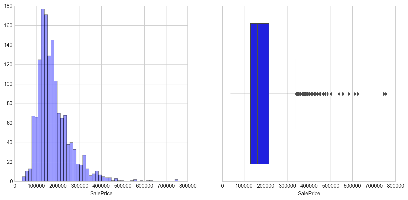
The dependent variable looks to be right skewed due to several high valued houses. The boxplot shows the presence of outliers beyond $340,000. For the purpose of linear regression, we do not have to assume that our dependent variable follows a normal distribution. We will however keep in mind the fact that we might want to do some outlier processing to improve regression results.
Initial cleaning of data
Before we dive deeper into the features, we will perform some preprocessing work. They include:
- Cleaning the column headers and index
- Checking for duplicates
- Checking for negative numbers
- Removing non-residential houses
- Handling the null values
1. Cleaning column headers and index
Column headers look fine except that I prefer to work with small caps. Let’s define a function to transform them.
def clean_columns(df):
    df.columns = [x.lower() for x in df.columns]
    return df
clean_columns(house)
The id column is unique to each house and can be set as the index.
house.set_index('id', inplace=True )
2. Check for duplicates
We now look for any repeat observations in our data
house.duplicated().sum()
0
Looks like there aren’t any
3. Check for negative numbers
Taking a look at the data dictionary, there doesn’t seem to be any reason for negative numbers. Let’s check if there are any in our dataset
house.lt(0).sum().sum()
0
Just as expected.
4. Remove non-residential houses
Looking at the mszoning feature, there seems to be some buildings in our dataset that could belong to non-residential types including commercial and industrial types. Let’s take a look at the distribution of housing types in our dataset.
house['mszoning'].value_counts()
RL         1151
RM          218
FV           65
RH           16
C (all)      10
Name: mszoning, dtype: int64
It seems that other than 10 commercial buildings, the other types are residential. We will remove these 10 commercial buildings to narrow our model predictive ability to only residential building types.
house = house.loc[house['mszoning'] != 'C (all)',:]
house.shape
(1450, 80)

#Reset index and drop id column
house.reset_index(drop=True, inplace=True)
house.drop('id', axis=1, inplace=True)
5. Handle Null values
As a rule of thumb, features with more than 70% null values should be dropped as imputing them with artificial values will not be a good representation of the actual observations.
In this case, we will drop features that have more than 1020 null values
house.isnull().sum().sort_values(ascending=False)
poolqc           1443
miscfeature      1398
alley            1361
fence            1172
fireplacequ       681
lotfrontage       259
garagetype         79
garagecond         79
garagefinish       79
garagequal         79
garageyrblt        79
bsmtfintype2       38
bsmtexposure       38
bsmtqual           37
bsmtcond           37
bsmtfintype1       37
masvnrarea          8
masvnrtype          8
electrical          1
--- Truncated ---
There are 4 features that do not fulfill our criteria of less than 70% NaNs. I decided to drop those 4 as they will not be useful as predictors. A further check also showed that poolarea is highly correlated to poolqc and only has values for the same 7 houses, the rest are 0. We will drop that feature too.
house.drop(['poolqc', 'miscfeature', 'alley', 'fence', 'poolarea'], axis=1, inplace=True)
house.shape
(1450, 75)
Let’s go down the list of the other features to determine how we will impute the NaN values.
house['fireplacequ'].unique()
array([nan, 'TA', 'Gd', 'Fa', 'Ex', 'Po'], dtype=object)
The nan values in fireplacequ indicates that a house does not have a fireplace. We will impute those with ‘NA’
house['fireplacequ'].fillna('NA', inplace=True)
The lot frontage is next in line
house['lotfrontage'].describe()
count    1191.000000
mean       70.052897
std        24.301013
min        21.000000
25%        59.000000
50%        70.000000
75%        80.000000
max       313.000000
Name: lotfrontage, dtype: float64
Seeing as to how the feature looks to be normally distributed (mean and median are very similar), we will impute with the median value.
house['lotfrontage'].fillna(house['lotfrontage'].median(), inplace = True)
Now we look at the null values in the garage
house['garagecond'].unique()
array(['TA', nan, 'Gd', 'Fa', 'Po', 'Ex'], dtype=object)

house['garagetype'].unique()
array(['Attchd', 'Detchd', 'BuiltIn', 'CarPort', nan, 'Basment', '2Types'], dtype=object)

house['garagefinish'].unique()
array(['RFn', 'Unf', 'Fin', nan], dtype=object)

house['garagequal'].unique()
array(['TA', 'Fa', 'Gd', nan, 'Ex', 'Po'], dtype=object)

house['garageyrblt'].unique()
array([ 2003.,  1976.,  2001.,  1998.,  2000.,  1993.,  2004.,  1973.,
        1931.,  1939.,  1965.,  2005.,  1962.,  2006.,  1960.,  1991.,
        1970.,  1967.,  1958.,  1930.,  2002.,  1968.,  2007.,  2008.,
        1957.,  1920.,  1966.,  1959.,  1995.,  1954.,  1953.,    nan,
        1983.,  1977.,  1997.,  1985.,  1963.,  1981.,  1964.,  1999.,
        1935.,  1990.,  1945.,  1987.,  1989.,  1915.,  1956.,  1948.,
        1974.,  2009.,  1950.,  1961.,  1921.,  1979.,  1951.,  1969.,
        1936.,  1975.,  1971.,  1923.,  1984.,  1926.,  1955.,  1986.,
        1988.,  1916.,  1932.,  1972.,  1918.,  1980.,  1924.,  1996.,
        1940.,  1949.,  1994.,  1910.,  1978.,  1982.,  1992.,  1925.,
        1941.,  2010.,  1927.,  1947.,  1937.,  1942.,  1938.,  1952.,
        1928.,  1922.,  1934.,  1906.,  1914.,  1946.,  1908.,  1929.,
        1933.])
Similar to the fireplace, we will impute ‘NA’ for houses without garage. The only exception is the garageyrblt where we will impute with the median year.
house['garagecond'].fillna('NA', inplace=True)
house['garagetype'].fillna('NA', inplace=True)
house['garageyrblt'].fillna(house['garageyrblt'].median(), inplace=True)
house['garagefinish'].fillna('NA', inplace=True)
house['garagequal'].fillna('NA', inplace=True)
Next we look at the null values in the basement
house['bsmtexposure'].unique()
array(['No', 'Gd', 'Mn', 'Av', nan], dtype=object)

house['bsmtfintype2'].unique()
array(['Unf', 'BLQ', nan, 'ALQ', 'Rec', 'LwQ', 'GLQ'], dtype=object)

house['bsmtfintype1'].unique()
array(['GLQ', 'ALQ', 'Unf', 'Rec', 'BLQ', nan, 'LwQ'], dtype=object)

house['bsmtcond'].unique()
array(['TA', 'Gd', nan, 'Fa', 'Po'], dtype=object)

house['bsmtqual'].unique()
array(['Gd', 'TA', 'Ex', nan, 'Fa'], dtype=object)
The values are all ordinal in nature. We will impute ‘NA’ to all of them.
house['bsmtexposure'].fillna('NA', inplace=True)
house['bsmtfintype2'].fillna('NA', inplace=True)
house['bsmtfintype1'].fillna('NA', inplace=True)
house['bsmtcond'].fillna('NA', inplace=True)
house['bsmtqual'].fillna('NA', inplace=True)
Next up is the masonry veneer area and type
house['masvnrtype'].unique()
array(['BrkFace', 'None', 'Stone', 'BrkCmn', nan], dtype=object)

house['masvnrarea'].unique()
array([  1.96000000e+02,   0.00000000e+00,   1.62000000e+02,
         3.50000000e+02,   1.86000000e+02,   2.40000000e+02,
         2.86000000e+02,   3.06000000e+02,   2.12000000e+02,
         1.80000000e+02,   3.80000000e+02,   2.81000000e+02,
         6.40000000e+02,   2.00000000e+02,   2.46000000e+02,
         1.32000000e+02,   6.50000000e+02,   1.01000000e+02,
         4.12000000e+02,   2.72000000e+02,   4.56000000e+02,
         1.03100000e+03,   1.78000000e+02,   5.73000000e+02,
         3.44000000e+02,   2.87000000e+02,   1.67000000e+02,
         1.11500000e+03,   4.00000000e+01,   1.04000000e+02,
         5.76000000e+02,   4.43000000e+02,   4.68000000e+02,
         6.60000000e+01,   2.20000000e+01,   2.84000000e+02,
         ---Truncated---
Seeing as to how there is already a ‘None’ value in masvnrtype and a 0 value in masvnrarea, we will impute all missing values in masvnrtype to ‘None and that in masvnrarea to 0.
house['masvnrarea'].fillna(0, inplace=True)
house['masvnrtype'].fillna('None', inplace=True)
The final feature to consider for Null handling is the electrical column
house['electrical'].unique()
array(['SBrkr', 'FuseF', 'FuseA', 'FuseP', 'Mix', nan], dtype=object)
They are all unique values. We will impute with the mode for that single house that doesn’t have a value.
house['electrical'].fillna(house['electrical'].mode(), inplace=True)
house.isnull().sum().sum()
0
Great, now that all null values have been handled, we will look into feature engineering.
Feature Engineering
Now, let’s see if we can create some new features that can help us better explain the data.
We will take a look at year features, combining features that describe the same thing, area features, bathroom features, ordinal features, features rating the quality and condition and finally cyclical features.
Year features
Let’s first explore the features with year values. The age of the house, garage and its furnishings might be better able to explain the prices it was sold at. We will derive these values from the year they were commenced right up to when they were sold.
house['houseage'] = house['yrsold'] - house['yearbuilt']
house['garageage'] = house['yrsold'] - house['garageyrblt']
house['furnishage'] = house['yrsold'] - house['yearremodadd']
house.drop(['yearbuilt', 'garageyrblt', 'yearremodadd'], axis=1, inplace=True)
Combining features describing the same thing
Next we combine both condition1 and condition2 into one feature as they are referring to the same set of values.
house['condition'] = np.where(house['condition1'] == house['condition2'], house['condition1'], house['condition1'] + house['condition2'])
house.drop(['condition1', 'condition2'], axis=1, inplace=True)
We do the same for Exterior1st and Exterior 2nd
house['exterior'] = np.where(house['exterior1st'] == house['exterior2nd'], house['exterior1st'], house['exterior1st'] + house['exterior2nd'])
house.drop(['exterior1st', 'exterior2nd'], axis=1, inplace=True)
Area features
Next we look at the square feet measurements and see if we can engineer or remove some features
house[['bsmtfinsf1', 'bsmtfinsf2', 'bsmtunfsf', 'totalbsmtsf']].head()
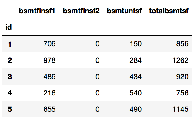
It looks like totalbsmtsf is a sum total of the other 3 columns. And it seems that bsmtinsf2 is very sparse. We will drop totalbsmtsf and combine bsmtfinsf1 and bsmtfinsf2 into a new feature.
house['bsmtfinsf'] = house['bsmtfinsf1'] + house['bsmtfinsf2']
house.drop(['bsmtfinsf1', 'bsmtfinsf2', 'totalbsmtsf'], axis=1, inplace = True)
Next we look at the square feet coverage of the house.
house[['1stflrsf', '2ndflrsf', 'lowqualfinsf', 'grlivarea']].tail(20)
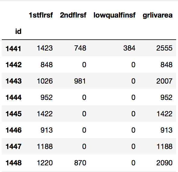 Truncated to show sum of 3 columns equals to grlivarea
It seems that grlivarea is comprised of the sum of the other 3 columns. Both 2ndflrsf and lowqualfinsf look considrably sparse. Let’s investigate.
house['2ndflrsf'].value_counts()
0       824
728      10
504       9
672       8
546       8
720       7
600       7
---Truncated---
house['lowqualfinsf'].value_counts()
0      1425
80        3
360       2
371       1
53        1
120       1
---Truncated---
Since both features are considerably sparse, I will drop them as well as the 1stflrsf column as they are all included in grlivarea and will be collinear.
house.drop(['1stflrsf', '2ndflrsf', 'lowqualfinsf'], axis=1, inplace=True)
Final area to look at is the porch
house[['wooddecksf', 'openporchsf', 'enclosedporch', '3ssnporch', 'screenporch']]
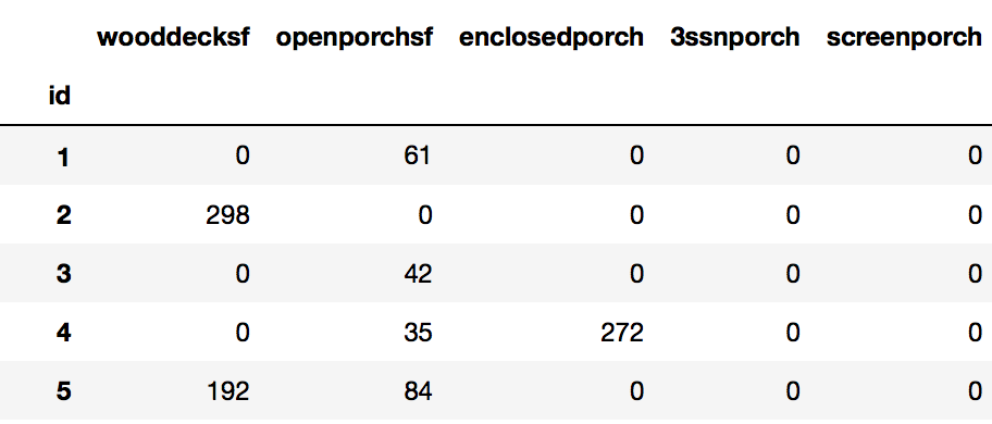
Upon performing value_counts(), all 5 features have considerable amount of 0 values. I will create a new porch feature to combine all of this data.
house['porch'] = house['wooddecksf'] + house['openporchsf'] + house['enclosedporch'] + house['3ssnporch'] + house['screenporch']
house.drop(['wooddecksf', 'openporchsf', 'enclosedporch', '3ssnporch', 'screenporch'], axis=1, inplace=True)
Bathroom features
Let’s now take a look at the bathroom features
house[['bsmtfullbath', 'fullbath', 'halfbath', 'bsmthalfbath']].head(20)
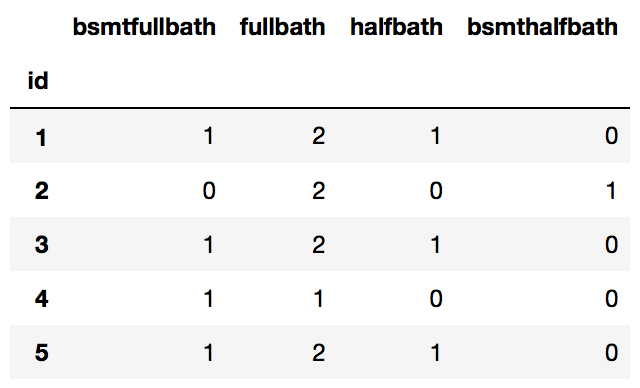
Both the halfbath features look to be rather sparse. Let’s investigate.
house['halfbath'].value_counts()
0    904
1    534
2     12
Name: halfbath, dtype: int64
house['bsmthalfbath'].value_counts()
0    1369
1      79
2       2
Name: bsmthalfbath, dtype: int64
Indeed they are and might not be useful predictors for us. Let’s combine all the bathrooms values into on bath feature indicating number of bathrooms in the house.
house['bath'] = house['bsmthalfbath'] + house['bsmtfullbath'] + house['halfbath'] + house['fullbath']
house.drop(['bsmthalfbath', 'bsmtfullbath', 'halfbath', 'fullbath'], axis=1, inplace=True)
Ordinal Features
Some of the features have an order to their values. An Excellent is definitely better than a Poor rating. We will encode these ordinal features to account for their difference in weights
six_ratings = lambda x: 5 if x=='Ex' else 4 if x=='Gd' else 3 if x=='TA' else 2 if x=='Fa' else 1 if x=='Po' else 0
five_ratings = lambda x: 5 if x=='Ex' else 4 if x=='Gd' else 3 if x=='TA' else 2 if x=='Fa' else 1
seven_ratings = lambda x: 6 if x=='GLQ' else 5 if x=='ALQ' else 4 if x=='BLQ' else 3 if x=='Rec' else 2 if x=='LWQ'\
else 1 if x=='Unf' else 0
house['exterqual'] = house['exterqual'].apply(five_ratings)
house['extercond'] = house['extercond'].apply(five_ratings)
house['bsmtqual'] = house['bsmtqual'].apply(six_ratings)
house['bsmtcond'] = house['bsmtcond'].apply(six_ratings)
house['bsmtfintype'] = house['bsmtfintype1'].apply(seven_ratings) + house['bsmtfintype2'].apply(seven_ratings)
house['bsmtexposure'] = house['bsmtexposure'].apply(lambda x: 4 if x=='Gd' else 3 if x=='Av' else 2 if x=='Mn' else 1 if x=="No" else 0)
house['heatingqc'] = house['heatingqc'].apply(five_ratings)
house['kitchenqual'] = house['kitchenqual'].apply(five_ratings)
house['fireplacequ'] = house['fireplacequ'].apply(six_ratings)
house['garagequal'] = house['garagequal'].apply(six_ratings)
house['garagecond'] = house['garagecond'].apply(six_ratings)
house.drop(['bsmtfintype1', 'bsmtfintype2'], axis=1, inplace=True)
We drop bsmtfintype1 and 2 as they have been combined to form a single bsmtfintype feature.
Quality and Condition
There are several features that are rated on the quality and condition. Let’s take a look at these features to decide if we should take any action.
We first perform chi2 tests of independence to look for any correlation between these categorical variables.
from scipy.stats import chi2_contingency
observed = pd.crosstab(house['overallqual'], house['overallcond'])
chi2_contingency(observed)
1224.807874384609,
 3.9260754195024299e-209
 ---Truncated---
The second value, the P-value, tells us that we should reject the null hypothesis that there is no relationship between the variables. We will combine the features into one that is the sum of the values.
house['overallqualcond'] = house['overallqual'] + house['overallcond']
house.drop(['overallqual', 'overallcond'], axis=1, inplace=True)
Let’s now do the same with garage, basement and exterior
observed = pd.crosstab(house['garagequal'], house['garagecond'])
chi2_contingency(observed)
3618.5201510975894,
 0.0
 ---Truncated---
observed = pd.crosstab(house['bsmtqual'], house['bsmtcond'])
chi2_contingency(observed)
1621.616686005882,
0.0
---Truncated---
observed = pd.crosstab(house['extercond'], house['exterqual'])
chi2_contingency(observed)
149.82854810419238,
 6.1426177291591305e-26
 ---Truncated---
The P-values for all 3 are less than 0.05 which means we reject the null hypothesis that there is no relationship between the variables. Let’s combine each pair into one feature and drop the individual features from our dataset.
house['extercondqual'] = house['extercond'] + house['exterqual']
house['garagecondqual'] = house['garagecond'] + house['garagequal']
house['bsmtcondqual'] = house['bsmtcond'] + house['bsmtqual']
house.drop(['extercond', 'exterqual', 'garagecond', 'garagequal', 'bsmtcond', 'bsmtqual'], axis=1, inplace=True)
Cyclical Features
The month sold variable is cyclical in nature as december is close to january and not as far apart as 1 is from 12. Let’s map observations onto a circle and compute x- and y- components of that point using sin and cos functions
house['mosold_sin'] = np.sin((house['mosold']-1) * (2. * np.pi/12))
house['mosold_cos'] = np.cos((house['mosold']-1) * (2. * np.pi/12))
house.drop('mosold', axis=1, inplace=True)
house.shape
(1450, 57)
Through this stage of feature engineering, we have reduced our feature set to 57. We will next look at filter methods of feature selection to further reduce the number of dimensions in our dataset.
Feature Selection - Filter methods
Next we select a subset of the features that best explains the target variable, which in our case, is the saleprice. We do so by performing the following tests on our feature set
- Pearson Correlation (Check for multicollinearity)
- Variance Inflation Factor (Check for multicollinearity)
- Eliminate features with low variance
First, we extract out our numeric variables
continuous_features = house._get_numeric_data()
continuous_features.shape
(1450, 32)
1. Pearson Correlation
We will be using the yellowbrick package for visualization.
from yellowbrick.features.rankd import Rank2D, Rank1D
y = continuous_features['saleprice']
X = continuous_features.drop(['saleprice'], axis=1)
plt.figure(figsize=(10,10))
visualizer = Rank2D()
visualizer.fit(X,y)
visualizer.transform(X)
visualizer.poof()
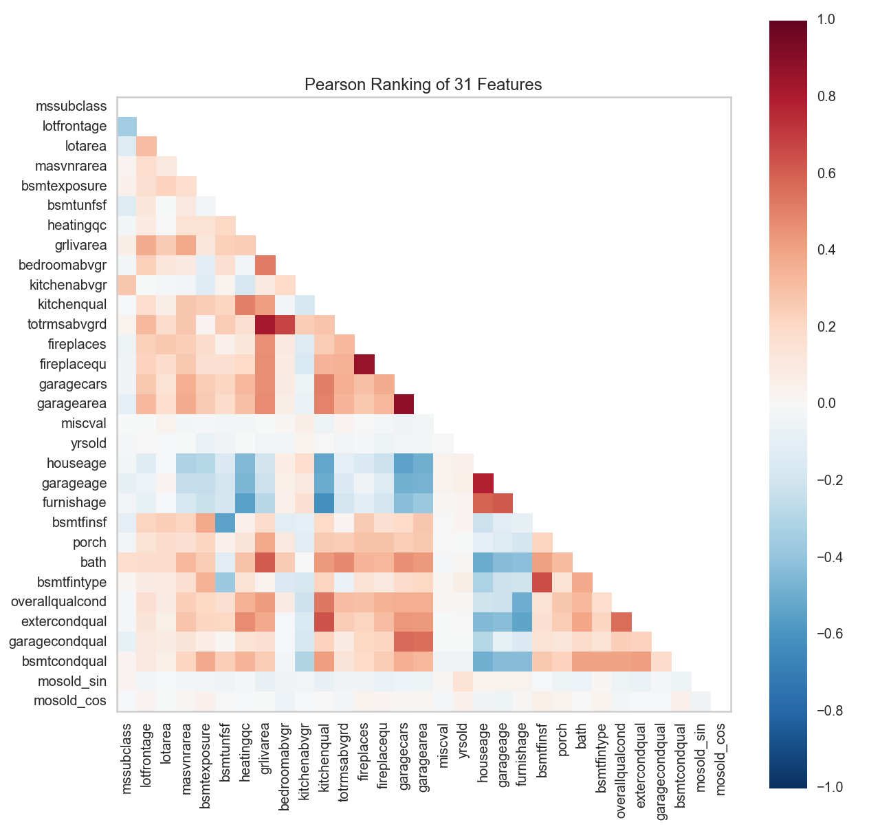
We can see firstly that garagecars and garagearea are highly correlated. We will drop garagecars as it looks to have higher correlation with other variables. Next, we can observe that fireplacequ and fireplaces are also highly correlated. We will drop fireplacequ as it too looks to have higher correlation with other variables. houseage and garageage look to be rather highly correlated too. We will drop houseage in favour of the other variable with lower correlation to other predictors. Finally, totrmsabvdrd looks to be highly correlated with grlivarea and bedroomabvgr. Let’s investigate!
house.drop(['garagecars', 'fireplacequ', 'houseage'], axis=1, inplace=True)
observed = pd.crosstab(house['totrmsabvgrd'], house['bedroomabvgr'])
chi2_contingency(observed)
2976.3876070778488,
 0.0
 ---Truncated---
It seems reasonable enough to understand why a relationship is observed between number of bedrooms above grade and total number of rooms above grade, which is further proven by the significant chi2 test result. Let’s look at the relationship between totrmsabvgrd, a categorical variable, and the grlivarea, a continuous one using an ANOVA one-way test.
from scipy import stats
import statsmodels.api as sm
from statsmodels.formula.api import ols

mod = ols('grlivarea ~ totrmsabvgrd',
                data=house).fit()

aov_table = sm.stats.anova_lm(mod, typ=2)
print aov_table
                   sum_sq      df            F  PR(>F)
totrmsabvgrd  2.721091e+08     1.0  3090.157687     0.0
Residual      1.275061e+08  1448.0          NaN     NaN
There is a significant relationship between both variables as evidenced by the low p-value of the ANOVA test. We’ll drop totrmsabvgrd as a potential predictor.
house.drop('totrmsabvgrd', axis=1, inplace=True)
2. Variance Inflation Factor
The Variance Inflation Factor (VIF) checks to see if any of the features in a dataset tends to exhibit multicollinearity with other variables. This is accomplished through an analysis of how ‘inflated’ the variance of the coefficient of a feature becomes in comparison to the other features in a multiple linear regression. A VIF more than 5 indicates high correlation while values between 1-5 show moderate correlation.
#We need to reset our continuous features and X as we have dropped some variables
continuous_features = house._get_numeric_data()
X = continuous_features.drop('saleprice', axis=1)

#We need to standardize our features first
from sklearn.preprocessing import StandardScaler

scaler = StandardScaler()
Xs = scaler.fit_transform(X)

from statsmodels.stats.outliers_influence import variance_inflation_factor

VIF = [(continuous_features.columns[i], variance_inflation_factor(Xs, i)) for i in range(Xs.shape[1])]

VIF_df = pd.DataFrame(list(zip(*VIF)[1]), index = list(zip(*VIF)[0]))

fig, ax = plt.subplots()
VIF_df.plot(kind = 'bar', legend = False, ax = ax)
ax.axhline(5, c = 'r', lw = 3)
ax.text(5, 5.2, 'If VIF is above this boundary, column is multi-collinear')
plt.show()
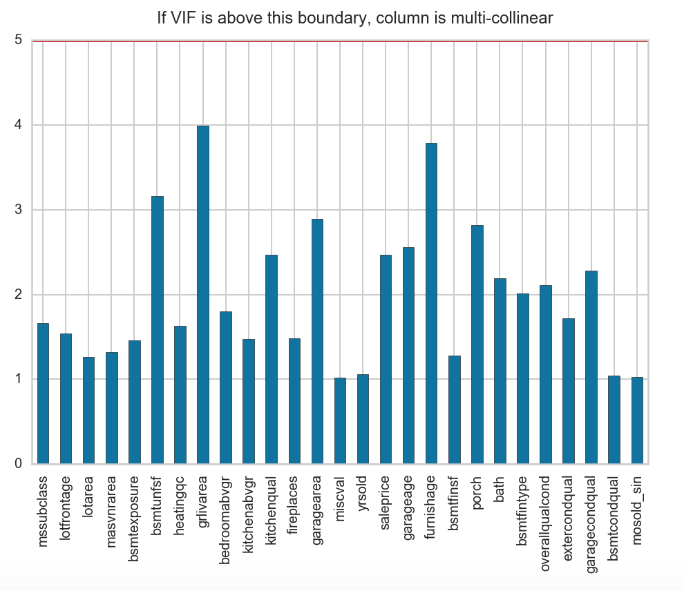
It would seem that none of our other features are highly correlated with each other although several features are moderately correlated.
3. Low Variance Check
We next identify features with low or near zero variance through the following function. Near zero variance features are qualified as those with a 19x difference in the highest value to the next highest value including having the total number of distinct values to be less than 10% of the total number of samples.
Here’s a function that accomplishes this check
def nearZeroVariance(X, freqCut = 95 / 5, uniqueCut = 5):
    '''
    Determine predictors with near zero or zero variance.
    Inputs:
    X: pandas data frame
    freqCut: the cutoff for the ratio of the most common value to the second most common value
    uniqueCut: the cutoff for the percentage of distinct values out of the number of total samples
    Returns a tuple containing a list of column names: (zeroVar, nzVar)
    '''

    colNames = X.columns.values.tolist()
    freqRatio = dict()
    uniquePct = dict()

    for names in colNames:
        counts = (
            (X[names])
            .value_counts()
            .sort_values(ascending = False)
            .values
            )

        if len(counts) == 1:
            freqRatio[names] = -1
            uniquePct[names] = (float(len(counts)) / len(X[names])) * 100
            continue

        freqRatio[names] = counts[0] / counts[1]
        uniquePct[names] = (float(len(counts)) / len(X[names])) * 100

    zeroVar = list()
    nzVar = list()
    for k in uniquePct.keys():
        if freqRatio[k] == -1:
            zeroVar.append(k)

        if uniquePct[k] < uniqueCut and freqRatio[k] > freqCut:
            nzVar.append(k)

    return(zeroVar, nzVar)
We will put our entire feature set into the function.
X = house.drop('saleprice', axis=1)
zeroVar, nzVar = nearZeroVariance(X)
print zeroVar, nzVar
[] ['landslope', 'functional', 'kitchenabvgr', 'roofmatl', 'street', 'landcontour', 'miscval', 'utilities', 'heating']
These are the featrues that are identified to have low variance. Let’s take a look at their distribution.
features = house.loc[:, ['landslope', 'functional', 'kitchenabvgr', 'roofmatl', 'street', 'landcontour', 'miscval',
                         'utilities', 'heating']]

fig, ax = plt.subplots(nrows=3, ncols = 3, figsize = (16,16))

for idx, col_name in enumerate(features.columns):
    row = int(idx / 3)
    col = int(idx % 3)
    ax[row][col].set_title(col_name)
    ax[row][col].hist(house[col_name].factorize()[0])

plt.tight_layout()

fig.patch.set_facecolor('white')
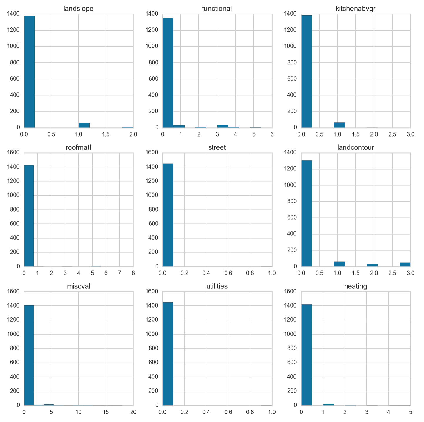
We can indeed observe the high prevalence for one value, the 0 value, and minimal contribution by the others. We will drop these features from our dataset.
house.drop(['landslope', 'functional', 'kitchenabvgr', 'roofmatl', 'street', 'landcontour', 'miscval', 'utilities', 'heating'], axis=1, inplace=True)
house.shape
(1450, 44)
By performing a series of feature engineering and feature selection, we have reduced our feature set from 81 variables to the 44 currently.
In part 2, we will further process the data in order to efficiently create a model that can predict housing prices based on features of property sold previously. In particular, we will identify what are the non-renovatable features of a house that can be used to predict the value of a house and what renovations can best explain the variance in price on the actual selling price of a property and its predicted value.
The repo for this series can be found here