With our dataset preprocessed from 81 features to the 44 that we have currently in part 1, we will now model our dataset with a variety of regression models to identify the best model to predict housing prices.
We will actually split our dataset into 2 smaller dataframes, one with fixed features, features that are non-renovatable like the square area of the property or the neighborhood it is located, and the other with renovatable features like the quality and condition of different aspects of the house.
Setting up X and y
We want to setup our predictor and dependent variables for modeling and we will be training on pre 2010 data and predicting the saleprices of houses sold in 2010.
Here’s the list of fixed features that I have identified. As before, the data description text file will prove to be very handy in following along.
fixed_features = ['mssubclass', 'mszoning', 'lotfrontage', 'lotarea', 'lotshape', 'lotconfig', 'neighborhood', 'bldgtype', 'housestyle', 'masvnrarea','foundation','bsmtunfsf','grlivarea', 'bedroomabvgr', 'fireplaces', 'garagetype', 'mosold_sin', 'mosold_cos', 'furnishage', 'condition', 'garagearea', 'yrsold', 'garageage', 'bsmtfinsf', 'porch', 'bath']
print len(fixed_features)
26
We have 26 features that have been identified as non-renovatable ones. I should point out that the variables saletype and salecondition have been left out as predictors as they do not fit into either categories in predicting housing prices. They are describing the sale and would do little to help predict on unknown data.
Next we set up X_fixed and y_fixed with patsy. Patsy is utilized much like an R glm function and quickly generates our predictor dataframe with dummy variables encoded for categorical features as well as the dependent variable.
import patsy

house_fixed = house.loc[:, house.columns.isin(fixed_features)]

formula = 'saleprice ~ '+' + '.join([c for c in house_fixed.columns]) + ' -1'
print formula
y_fixed, X_fixed = patsy.dmatrices(formula, data=house, return_type='dataframe')
y_fixed = y_fixed.values.ravel()
print X_fixed.shape, y_fixed.shape

saleprice ~ mssubclass + mszoning + lotfrontage + lotarea + lotshape + lotconfig + neighborhood + bldgtype + housestyle + masvnrarea + foundation + bsmtunfsf + grlivarea + bedroomabvgr + fireplaces + garagetype + garagearea + yrsold + garageage + furnishage + condition + bsmtfinsf + porch + bath + mosold_sin + mosold_cos -1
(1450, 90) (1450,)
We can see that Patsy dmatrices has expanded the number of features from 26 to 90 to include dummy variables for all categorical columns.
Next we train-test split according to our year of sale criteria.
X_fixed_train = X_fixed.loc[house['yrsold'] != 2010,:]
X_fixed_test = X_fixed.loc[house['yrsold'] == 2010, :]
y_fixed_train = y_fixed[house['yrsold'] != 2010]
y_fixed_test = y_fixed[house['yrsold'] == 2010]
print 'Test set percentage of data: {0:.2f}'.format(float(y_fixed_test.shape[0])/y_fixed.shape[0] * 100)+'%'

Test set percentage of data: 11.86%
Modeling
Since our dependent variable is a continuous one, we will be utilizing regression models for our prediction task.
We will be performing linear regression on the fixed features first to get a baseline R2 score. Then we will perform regression with regularization to improve prediction accuracy through the wrapper methods of feature selection. These include ridge, lasso and elastic net regression models.
Next, we explore a stochastic gradient descent regressor method using gridsearch and finally we model with a decision tree regressor using gradient boosting with gridsearch over its hyperparameters.
Before all these though, we first create a function that will allow us to easily print out the RMSE evaluation metric for each model, the R2 accuracy, as well as either a plot of coefficient scores or feature importances.
from sklearn.preprocessing import StandardScaler
def model(clf, X_train, X_test, y_train, y_test, bar_plot=True):
    ss=StandardScaler()
    Xs_train = ss.fit_transform(X_train)
    Xs_test = ss.fit_transform(X_test)

    model = clf.fit(Xs_train, y_train)
    yhat = model.predict(Xs_test)

    print 'Model Report:'
    print 'RMSE: ', np.sqrt(metrics.mean_squared_error(y_test, yhat))
    print 'Accuracy: ', metrics.r2_score(y_test, yhat)
    if bar_plot ==True:
        try:
            feat_imp = pd.Series(clf.feature_importances_, X_train.columns).sort_values(ascending=False)
            fig, ax = plt.subplots(figsize=(13,8))
            feat_imp.head(40).plot(kind='bar', title='Feature Importance', ax=ax)
            plt.ylabel('Feature importance score')

        except AttributeError:
            coef_ranking = pd.Series(abs(clf.coef_), X_train.columns).sort_values(ascending=False)
            fig, ax = plt.subplots(figsize=(13,8))
            coef_ranking.head(40).plot(kind='bar', title='Coefficient Ranking', ax=ax)
            plt.ylabel('Coefficient Scores')
Our scaler of choice is a Standard Scaler where we normalize each feature to 0 mean and a standard deviation of 1. It is included in our ‘model’ function.
Linear Regression
Let’s start with our baseline model, linear regression.
from sklearn.linear_model import LinearRegression
from sklearn import metrics
model(LinearRegression(), X_fixed_train, X_fixed_test, y_fixed_train, y_fixed_test, bar_plot=False)

Model Report:
RMSE:  3.85742763419e+14
Accuracy:  -2.34054016647e+19
The negative R2 score of our linear regression suggests that our model still has features that are multicollinear.
Ridge Regression
Ridge introduces a regularization parameter to shrink the coefficients of features that are insignificant and amplifies those that matter more. Its main purpose is to handle multicollinearity in our data.
from sklearn.linear_model import RidgeCV
alpha_range = np.logspace(-10, 5, 200)
ridgeregcv = RidgeCV(alphas=alpha_range, scoring='neg_mean_squared_error', cv=3)
model(ridgeregcv, X_fixed_train, X_fixed_test, y_fixed_train, y_fixed_test)

Model Report:
RMSE:  30884.5226301
Accuracy:  0.849961639539
We can see that the accuracy has significantly improved over the baseline linear regression model. Let’s take a look at the top 40 features it has ranked in terms of their coefficient scores.
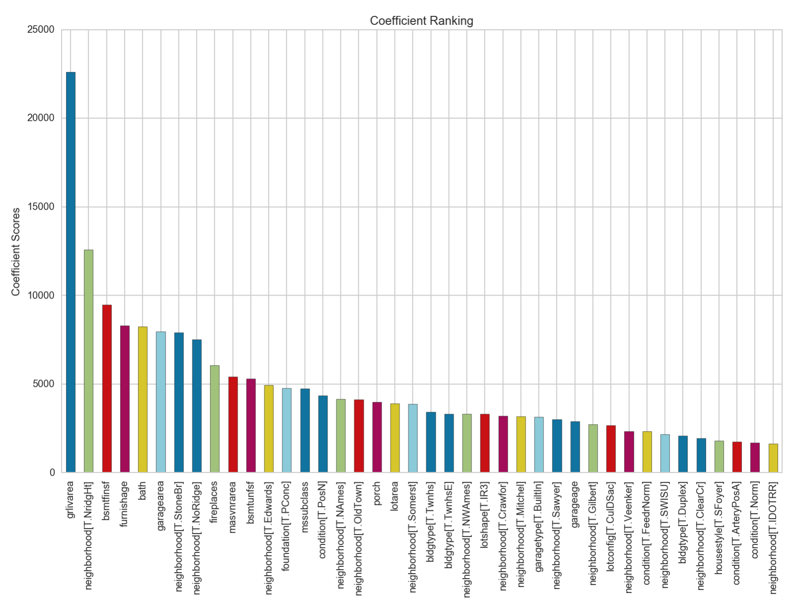
We can see that the coefficient with the greatest score, grlivarea, is about 2x more in magnitude than the coefficient with the 2nd largest value. We also note that there are several neighbourhood features that are deemed to be of significant contribution to the model.
Lasso Regression
Similar to Ridge, Lasso regression helps in solving the multicollinearity problem by shrinking coefficients of unwanted features. It does so more brutally by making them 0. Like Ridge, we will be using the cross-validated version of the algorithm here.
from sklearn.linear_model import LassoCV
lassoregcv = LassoCV(n_alphas=100)
model(lassoregcv, X_fixed_train, X_fixed_test, y_fixed_train, y_fixed_test)

Model Report:
RMSE:  30729.9549562
Accuracy:  0.851459674557
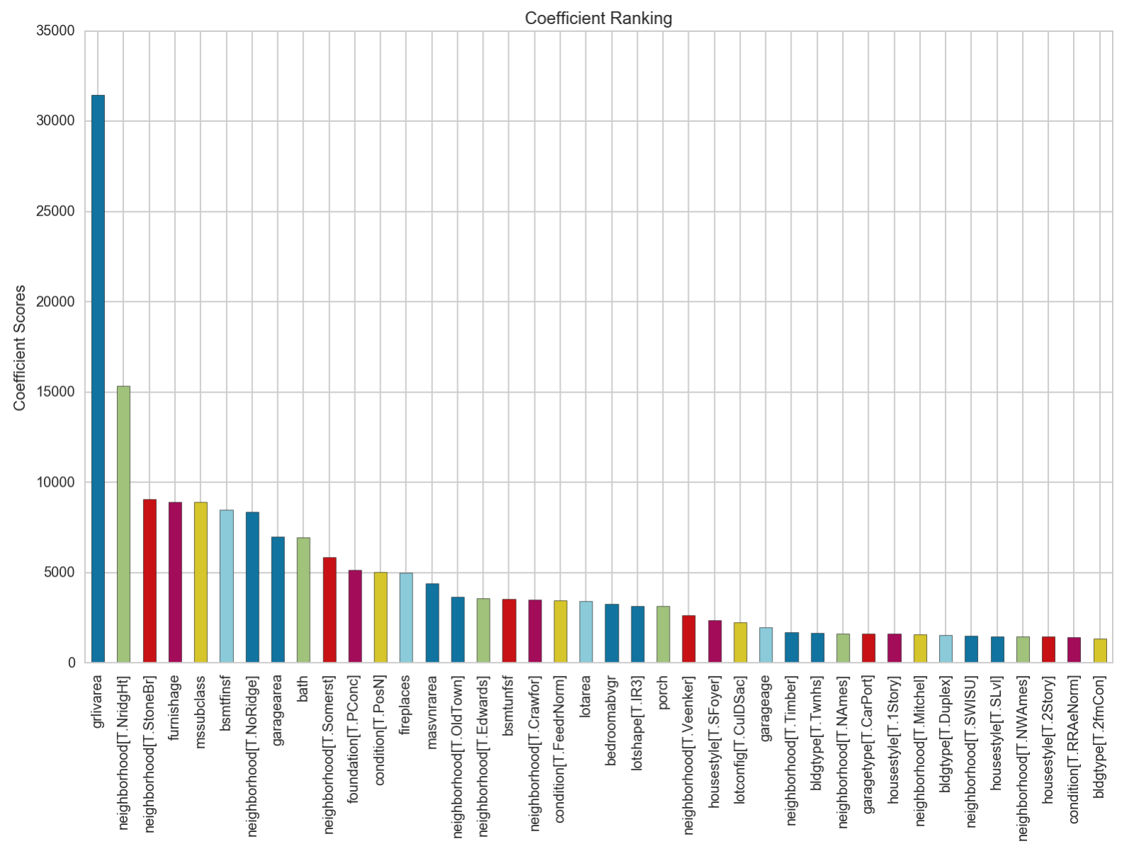
The values of the coefficients in the lasso regression model are higher than those in the ridge as several coefficients have been reduced to 0. grlivarea tops out at 31,000, compared to 23,000 in ridge. The proportion of differences between the top 40 coefficients also look to be similar to that of the Ridge regression.
lasso_coefs['variable'].loc[lassoregcv.coef_ == 0]
0                mszoning[FV]
1                mszoning[RH]
2                mszoning[RL]
3                mszoning[RM]
6             lotshape[T.Reg]
11    neighborhood[T.Blueste]
13    neighborhood[T.BrkSide]
18    neighborhood[T.Gilbert]
20    neighborhood[T.MeadowV]
30    neighborhood[T.SawyerW]
42       housestyle[T.2.5Unf]
46       foundation[T.CBlock]
48         foundation[T.Slab]
49        foundation[T.Stone]
52      garagetype[T.Basment]
55       garagetype[T.Detchd]
56           garagetype[T.NA]
61     condition[T.FeedrRRAn]
62     condition[T.FeedrRRNn]
64      condition[T.PosANorm]
66      condition[T.PosNNorm]
69      condition[T.RRAnNorm]
70      condition[T.RRNeNorm]
71     condition[T.RRNnFeedr]
74                lotfrontage
88                 mosold_sin
Name: variable, dtype: object
This list of 26 features that have their coefficients set to 0 shows that they exhibit correlation with other features in our dataset. While this tries to reduce multicollinearity, it does not mean that these features are not important in predicting the dependent variable. The arbitrary dropping of a feature due to its high correlation with another feature provides us with less ability to correctly interpret feature importance in predicting for our dependent variable.
ElasticNet
Elastic Net is simply a combination of both the Lasso and Ridge penalties to the loss function.
from sklearn.linear_model import ElasticNetCV, ElasticNet
l1_ratios = np.linspace(0.01, 1.0, 25)
optimal_enet = ElasticNetCV(l1_ratio=l1_ratios, n_alphas=100, cv=3, random_state=123)
optimal_enet.fit(Xs_fixed_train, y_fixed_train)
print optimal_enet.alpha_
print optimal_enet.l1_ratio_

559.941054205
1.0

enet = ElasticNet(alpha=optimal_enet.alpha_, l1_ratio=optimal_enet.l1_ratio_)
model(enet, X_fixed_train, X_fixed_test, y_fixed_train, y_fixed_test, bar_plot=False)

Model Report:
RMSE:  30729.9549562
Accuracy:  0.851459674557
The results of the elastic net modeling, which is exactly the same as our lasso model, shows that our best model so far is a lasso regression one.
SGDRegressor with GridsearchCV
In this model, we perform a stochastic gradient descent routine to minimize the error function. Scikit learn provides a class that we can easily employ our model with. Performing a gridsearchCV over the hyperparameters helps us optimize for the model.
from sklearn.linear_model import SGDRegressor
from sklearn.model_selection import GridSearchCV
sgd_params = {'loss':['squared_loss','huber'],
              'penalty':['l1','l2'],
              'alpha':np.logspace(-5,1,100),
              'learning_rate': ['constant', 'optimal', 'invscaling']
}
#We scale our train and test set here to pass into our sgd regressor instance.
ss = StandardScaler()
Xs_fixed_train = ss.fit_transform(X_fixed_train)
Xs_fixed_test = ss.fit_transform(X_fixed_test)

sgd_reg = SGDRegressor(random_state=123)
sgd_reg_gs = GridSearchCV(sgd_reg, sgd_params, cv=4, verbose=False, iid=False)
sgd_reg_gs.fit(Xs_fixed_train, y_fixed_train)

print sgd_reg_gs.best_params_
print sgd_reg_gs.best_score_
sgd_reg = sgd_reg_gs.best_estimator_

{'penalty': 'l2', 'alpha': 0.2310129700083158, 'learning_rate': 'invscaling', 'loss': 'squared_loss'}
0.754707390276

model(sgd_reg, X_fixed_train, X_fixed_test, y_fixed_train, y_fixed_test, bar_plot=False)

Model Report:
RMSE:  32293.258896
Accuracy:  0.835962072955
The scores obtained are not as good as those from either Lasso or Ridge.
Gradient Boosting Regressor
n the gradient boosting regressor, several weak learners are added together to boost the accuracy of the model. Each learner has a high bias but low variance. By combining successive iterations of learners, the model is able to reduce the bias gradually while keeping variance low.
We will be using Sklearn’s implementation of the regressor and tuning its hyperparameters over several iterations of gridsearch.
from sklearn.ensemble import GradientBoostingRegressor
gbr_base = GradientBoostingRegressor(random_state=123)
gbr_base.fit(Xs_fixed_train, y_fixed_train)
model(gbr_base, X_fixed_train, X_fixed_test, y_fixed_train, y_fixed_test, bar_plot=False)

Model Report:
RMSE:  26878.083128
Accuracy:  0.886363693545
The base model, before tuning for its hyperparameters, already registers a better score than all the previous regression models.
We first tune for the number of estimators or trees. It should be noted that we do not select a large value here first as it will increase the computation time.
param_test1 = {'n_estimators':range(20,81,10)}
gsearch1 = GridSearchCV(estimator = GradientBoostingRegressor(max_features='sqrt',random_state=123),
                        param_grid = param_test1, n_jobs=-1,iid=False, cv=5)
gsearch1.fit(Xs_fixed_train, y_fixed_train)
gsearch1.best_params_, gsearch1.best_score_

({'n_estimators': 80}, 0.83516675370867444)
We input the best number of estimators into our next set of gridsearching where we try to find how many levels the tree should split into and also how many samples there should be at least in each node before splitting. These are tree-related hyperparameters that we will be attempting to set first.
param_test2 = {'max_depth':range(2,17,2), 'min_samples_split':range(2,17,2)}
gsearch2 = GridSearchCV(estimator = GradientBoostingRegressor(n_estimators=80, max_features='sqrt', random_state=123),
param_grid = param_test2,n_jobs=-1,iid=False, cv=5)
gsearch2.fit(Xs_fixed_train, y_fixed_train)
gsearch2.best_params_, gsearch2.best_score_

({'max_depth': 4, 'min_samples_split': 10}, 0.85355510340917784)
We continue tuning another aspect of the tree hyperparameter, the minimum number of samples in each leaf node, for the 3rd routine.
param_test3 = {'min_samples_leaf':range(2,11)}
gsearch3 = GridSearchCV(estimator = GradientBoostingRegressor(max_depth=4, min_samples_split=10, n_estimators=80, max_features='sqrt', random_state=123),
param_grid = param_test3, n_jobs=-1, iid=False, cv=5)
gsearch3.fit(Xs_fixed_train, y_fixed_train)
gsearch3.best_params_, gsearch3.best_score_

({'min_samples_leaf': 2}, 0.85572841187059367)
With our tree hyperparameters tuned, we now look at how many features the algorithm should consider at most when looking at splitting, as well as the loss function.
param_test4 = {'max_features': ['sqrt', 'log2'], 'loss': ['ls', 'lad', 'huber']}
gsearch4 = GridSearchCV(estimator = GradientBoostingRegressor(max_depth=4, min_samples_split=10, min_samples_leaf = 2, n_estimators=80, random_state=123),
param_grid = param_test4, n_jobs=-1, iid=False, cv=5)
gsearch4.fit(Xs_fixed_train, y_fixed_train)
gsearch4.best_params_, gsearch4.best_score_

({'loss': 'ls', 'max_features': 'sqrt'}, 0.85572841187059367)
The subsample hyperparameter indicates what percentage of all the samples should be used for each individual weak learner. Any value below the default of 1.0 results in Stochastic Gradient boosting, reducing variance but increasing bias.
param_test5 = {'subsample':[0.6,0.7,0.75,0.8,0.85,0.9]}
gsearch5 = GridSearchCV(estimator = GradientBoostingRegressor(max_depth=4, min_samples_split=10, min_samples_leaf = 2,max_features='sqrt', n_estimators=80, random_state=123),
param_grid = param_test5, n_jobs=-1, iid=False, cv=5)
gsearch5.fit(Xs_fixed_train, y_fixed_train)
gsearch5.best_params_, gsearch5.best_score_

({'subsample': 0.85}, 0.84356674993247494)
The final parameters we will be tuning are the learning rate and the n_estimators, 2 hyperparameters that are inversely related to each other. The learning rate has to decrease to reduce the effect of each estimator in the overall model as the number of estimators increase
param_test6 = {'learning_rate':[0.05, 0.01, 0.005, 0.001], 'n_estimators': [160, 800, 1600, 3200, 6400, 12800, 25600]}
gsearch6 = GridSearchCV(estimator = GradientBoostingRegressor(subsample=0.85, max_depth=4, min_samples_split=10, min_samples_leaf = 2,max_features='sqrt', random_state=123),
param_grid = param_test6, n_jobs=-1, iid=False, cv=5)
gsearch6.fit(Xs_fixed_train, y_fixed_train)
gsearch6.best_params_, gsearch6.best_score_

({'learning_rate': 0.005, 'n_estimators': 6400}, 0.86816654113842717)

gbr_best = GradientBoostingRegressor(max_depth=4, min_samples_split=10, min_samples_leaf = 2,max_features='sqrt', n_estimators=6400, subsample=0.85, learning_rate=0.005, random_state=123)
model(gbr_best, X_fixed_train, X_fixed_test, y_fixed_train, y_fixed_test)

Model Report:
RMSE:  24047.6741039
Accuracy:  0.909036601209
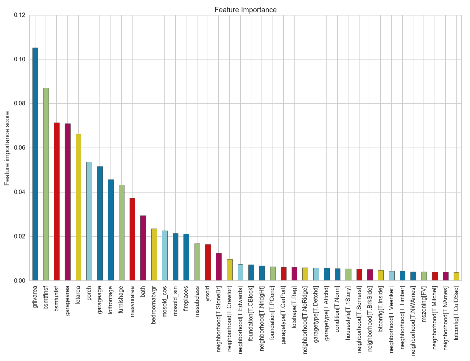
We can see that this provides us with the best accuracy score yet. The most important feature from this model is identified to be the area of the living area above ground. Let’s look at a plot of the residuals to see if this model fulfils the assumption of the homodasceity of its errors.
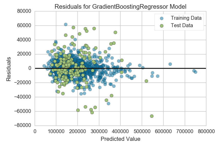
from yellowbrick.regressor.residuals import ResidualsPlot
visualizer = ResidualsPlot(gbr_best)
visualizer.fit(Xs_fixed_train, y_fixed_train)
visualizer.score(Xs_fixed_test, y_fixed_test)
visualizer.poof()
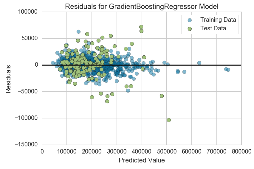
We can see that there does not seem to be a clear pattern forming that is characteristic of residuals with heterodasceity. Most values lie within +- 100,000, even for values that are on the higher end of the predicted vallues. There are a couple of points with high error values though that suggests the presence of outliers that can not be explained by the model.
from yellowbrick.regressor import PredictionError

visualizer = PredictionError(gbr_best)

visualizer.fit(Xs_fixed_train, y_fixed_train)
visualizer.score(Xs_fixed_test, y_fixed_test)
visualizer.poof()
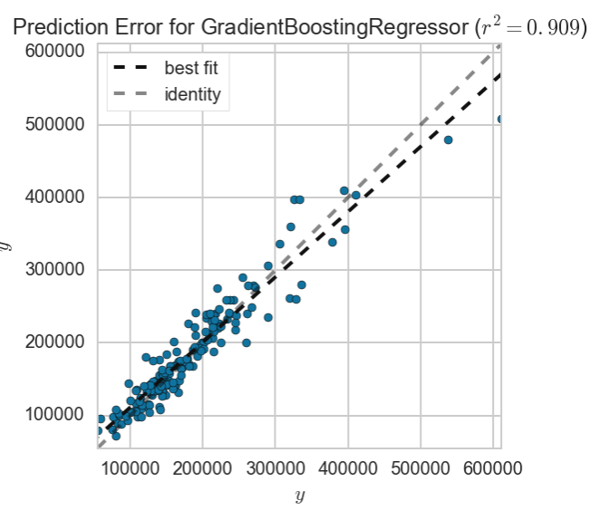
The prediction error line with the best fit shows that our gradient boosted linear model was able to predict most of the saleprices in our test set. We will now look at how we might want to remove some outliers to improve our model even further.
Outlier Handling
We look at our outliers at this point as we know what our most important feature is in predicting the saleprice. First we create a dataframe for all the fixed features including our saleprice. Doing so helped me realize that I needed to reset my index after dropping the 10 non-residential properties in part 1, which I have promptly gone back to edit.
y_fixed_series = pd.Series(y_fixed, name='saleprice')
fixed = X_fixed.join(y_fixed_series)
fixed.shape

(1450, 91)
We know that our most important feature is the living area above ground. Let’s analyze it against the dependent variable to see if we can detect any outliers
sns.jointplot(fixed['saleprice'], fixed['grlivarea'])
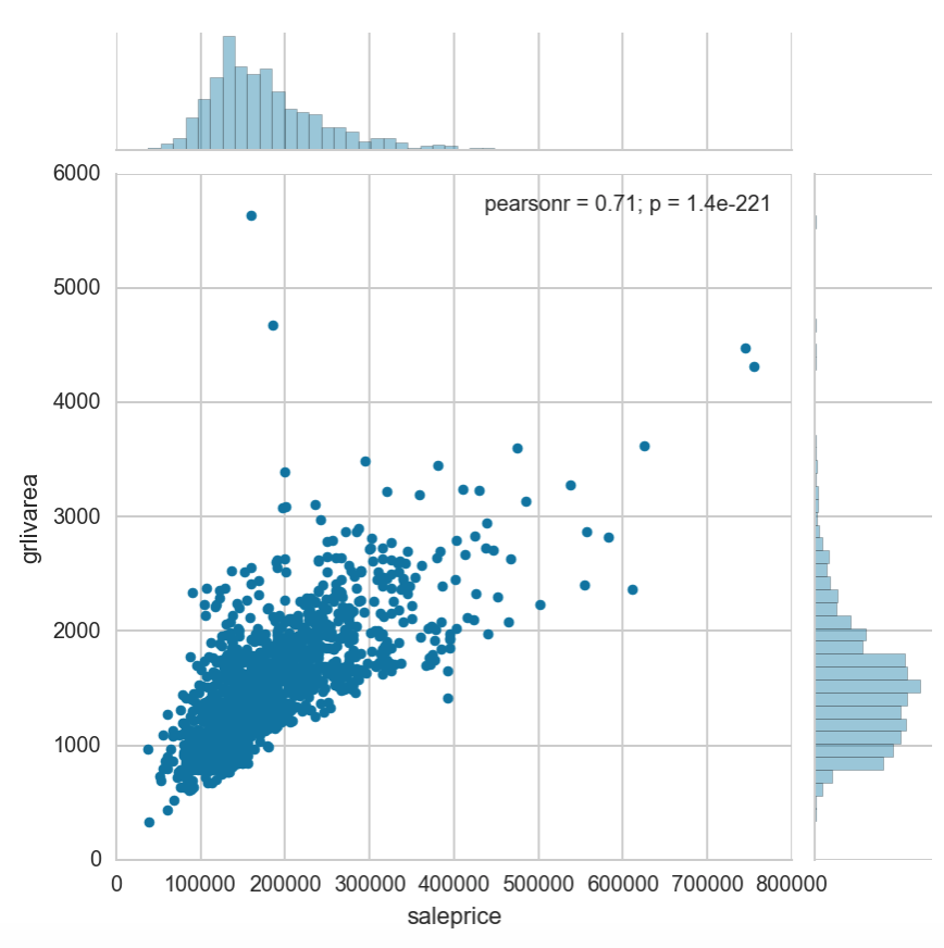
We can see that there is a strong correlation between grlivarea and the saleprice. There are however 2 properties that have large areas with saleprices that are too low for their size. We will attempt to drop them from our dataset and treat them as anomalies.
fixed.drop(index = fixed.loc[(fixed['grlivarea'] > 4000) & (fixed['saleprice'] < 200000)].index, inplace=True)
fixed.shape

(1448, 91)
X_fixed_out = fixed.iloc[:, :-1]
y_fixed_out = fixed['saleprice']

#Creating train and test sets without outlier
X_fixed_out_test = X_fixed_out.loc[fixed['yrsold'] == 2010, :]
X_fixed_out_train = X_fixed_out.loc[fixed['yrsold'] != 2010,:]
y_fixed_out_test = y_fixed_out[fixed['yrsold'] == 2010]
y_fixed_out_train = y_fixed_out[fixed['yrsold'] != 2010]
With our new training and test sets, let’s model them against our tuned gradient boosted regressor.
model(gbr_best, X_fixed_out_train, X_fixed_out_test, y_fixed_out_train, y_fixed_out_test)

Model Report:
RMSE:  21816.4924161
Accuracy:  0.925133009004
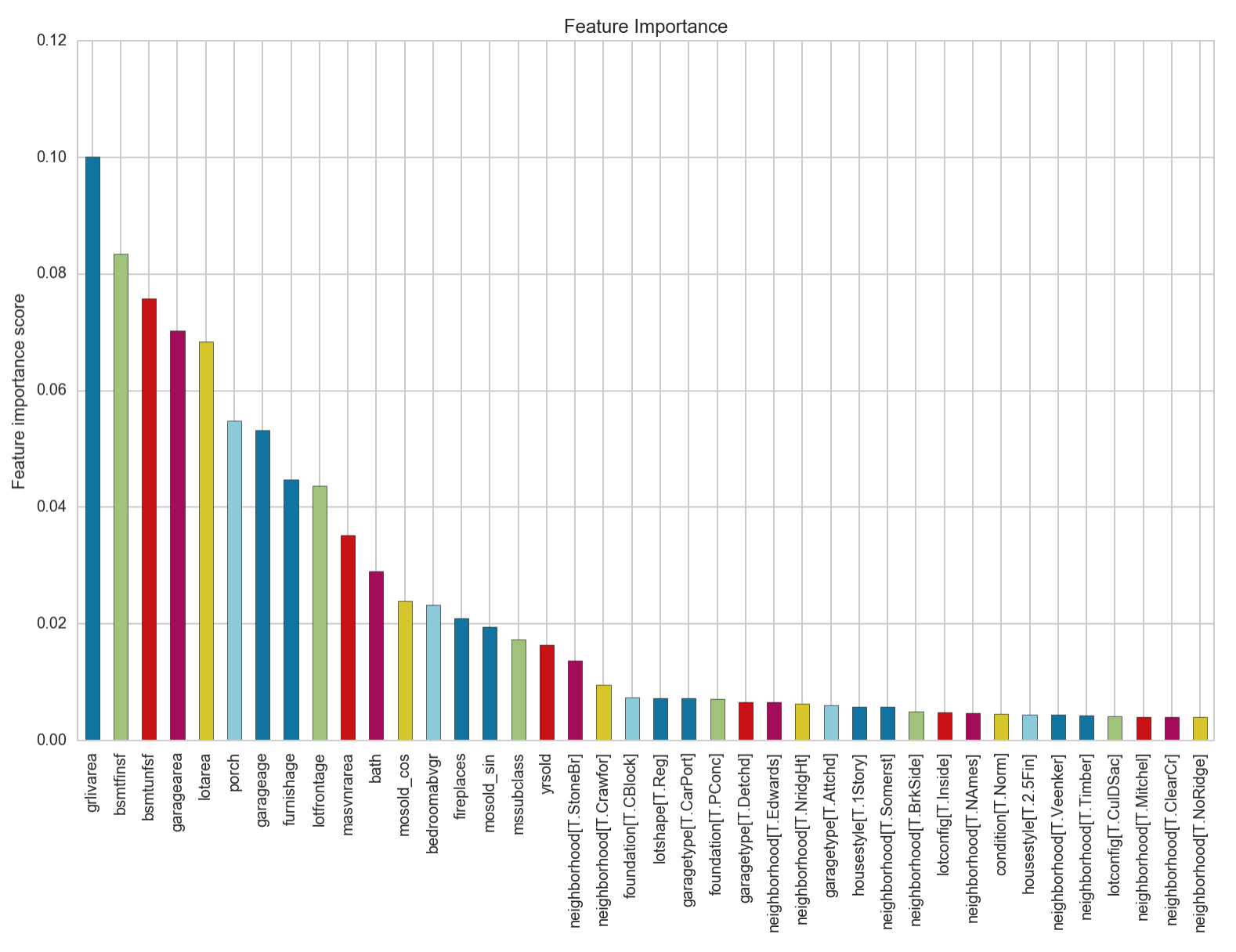
We can see that our accuracy has increased by 1.5%! The feature importance chart looks to not have changed from before the outlier removal. It seems that regardless of neighbourhood, the saleprice of a house is closely dependent on firstly, the area of the living area above ground, followed by the area of the basement, then the area of the surrounding vicinity including its garage, and porch. How old the garage is and when the house was furnished also features in contributing to the saleprice of a house.
Let’s take a look at the residuals and see how they compare against the previous plot
#Scaling is conducted outside of model function for our plotting functions
Xs_fixed_out_train = ss.fit_transform(X_fixed_out_train)
Xs_fixed_out_test = ss.fit_transform(X_fixed_out_test)

visualizer = ResidualsPlot(gbr_best)
visualizer.fit(Xs_fixed_out_train, y_fixed_out_train)
visualizer.score(Xs_fixed_out_test, y_fixed_out_test)
visualizer.poof()
The first thing we should notice is that the range of our residuals has shrunk to be bounded between +-70,000. The 2 outliers were contributing to quite a substantial amount of uncertainty in our model. Much like the plot before, we do not notice any noticeable pattern here which does not violate our assumption of homodasceitic errors in our model.
visualizer = PredictionError(gbr_best)

visualizer.fit(Xs_fixed_out_train, y_fixed_out_train)
visualizer.score(Xs_fixed_out_test, y_fixed_out_test)
visualizer.poof()
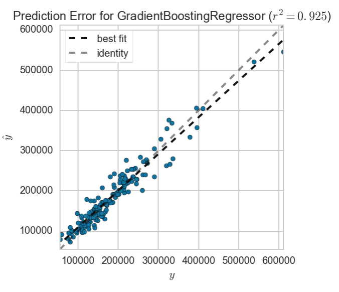
Finally, our best fit line looks to be even closer to the ideal fit line, suggesting that our model has a high degree of accuracy.
Model comparison and selection
| Model | R2 score |
|---|---|
| Linear Regression | -2.3405 |
| Ridge Regression | 0.8499 |
| Lasso Regression | 0.8515 |
| ElasticNet | 0.8515 |
| SGD Regressor | 0.8360 |
| Gradient Boosted Regressor | 0.9090 |
| Gradient Boosted Regressor w/o outliers | 0.9251 |
Judging by the R2 values alone, we will use the Gradient Boosted Regressor as our model of choice in predicting future prices of houses. We have to keep in mind that this model was developed solely on the fixed features of the house.
We have seen that the main criteria to look for in estimating the saleprice of a house in Ames is its living area above ground. Other area-related features like porch and basement square feet can and should be taken into consideration too.
This is only half the story however. We want to also investigate how much more the renovatable features contribute to the saleprice of a house and which are the most cost-efficient renovations that we can do to derive the most value. This will be covered in the final part of this 3-part series on predicting house prices with regression techniques
The repo for this series can be found here