Back in part 1, we preprocessed our housing data and performed some EDA on it. We then proceeded to model the fixed, non-renovatable features through a series of regression analyses in part 2.
In this final segment, we will attempt to analyze the impact the renovatable features have on the overall model by modeling to see how much these features can explain the variance we observe from our gradient boosted model using only the fixed features.
Our ultimate goal is to identify houses that are worth purchasing based on fixed features with a view to renovate for higher profits.
Modeling renovatable features to predict residuals from fixed features model
Our dependent variable for this piece of modeling work will be the residuals from the predicted saleprice from our fixed features model against the actual saleprice.
y_resid_test = y_test - gbr_best.predict(Xs_fixed_out_test)
y_resid_train = y_train - gbr_best.predict(Xs_fixed_out_train)
We next create our renovatable feature dataset that will be our set of predictors using patsy which automatically does the one-hot encoding for us. Just to recap, our set of renovatable features looks at the quality and condition of various aspecs of a house as well as facilities that can be easily upgraded like heating, exterior look, air conditioning etc.
renovatable_features = ['roofstyle','masvnrtype', 'bsmtexposure', 'heatingqc', 'centralair', 'electrical', 'kitchenqual', 'garagefinish', 'paveddrive', 'exterior', 'bsmtfintype', 'overallqualcond', 'extercondqual', 'garagecondqual', 'bsmtcondqual']

house_reno = house.loc[:, house.columns.isin(renovatable_features)]

formula = 'saleprice ~ '+' + '.join([c for c in house_reno.columns]) + ' -1'
print formula
_, X_reno = patsy.dmatrices(formula, data=house, return_type='dataframe')

saleprice ~ roofstyle + masvnrtype + bsmtexposure + heatingqc + centralair + electrical + kitchenqual + garagefinish + paveddrive + exterior + bsmtfintype + overallqualcond + extercondqual + garagecondqual + bsmtcondqual -1
We next create our train and test set for our predictors, which we have done earlier for our dependent variable.
X_reno_test = X_reno.loc[house['yrsold'] == 2010, :]
X_reno_train = X_reno.loc[house['yrsold'] != 2010,:]
Let’s model with Linear Regression to obtain a baseline gauge. We will use the model function defined in part 2.
model(LinearRegression(), X_reno_train, X_reno_test, y_resid_train, y_resid_test, bar_plot=False)

Model Report:
RMSE:  8.31115727018e+15
R2:  -1.47072440582e+23
The negative R2 value indicates that our regression line is worse than a horizontal line across the y-intercept.
We will model with a gradient boosted regressor. For the sake of brevity, I will leave out the hyperparameter tuning steps but you can refer to them in the accompanying jupyter notebook.
gbr_best_reno = GradientBoostingRegressor(max_depth=4, min_samples_split=22, min_samples_leaf = 4,max_features='sqrt', loss='huber', n_estimators=6400, subsample=0.75, learning_rate=0.001, random_state=123)
model(gbr_best_reno, X_reno_train, X_reno_test, y_resid_train, y_resid_test)

Model Report:
RMSE:  21050.8020685
R2:  0.0564919845084
As can be seen with our R2 score, our gradient boosted model only explains 5% of the variance seen in our predicted values of the dependent variable (residuals from fitted model) with the actual values.
While I would not trust using this model to identify the renovatable features that can explain the variance in predicted vs actual saleprice in our fitted model, I thought it was interesting to look at the output of the feature importance table.
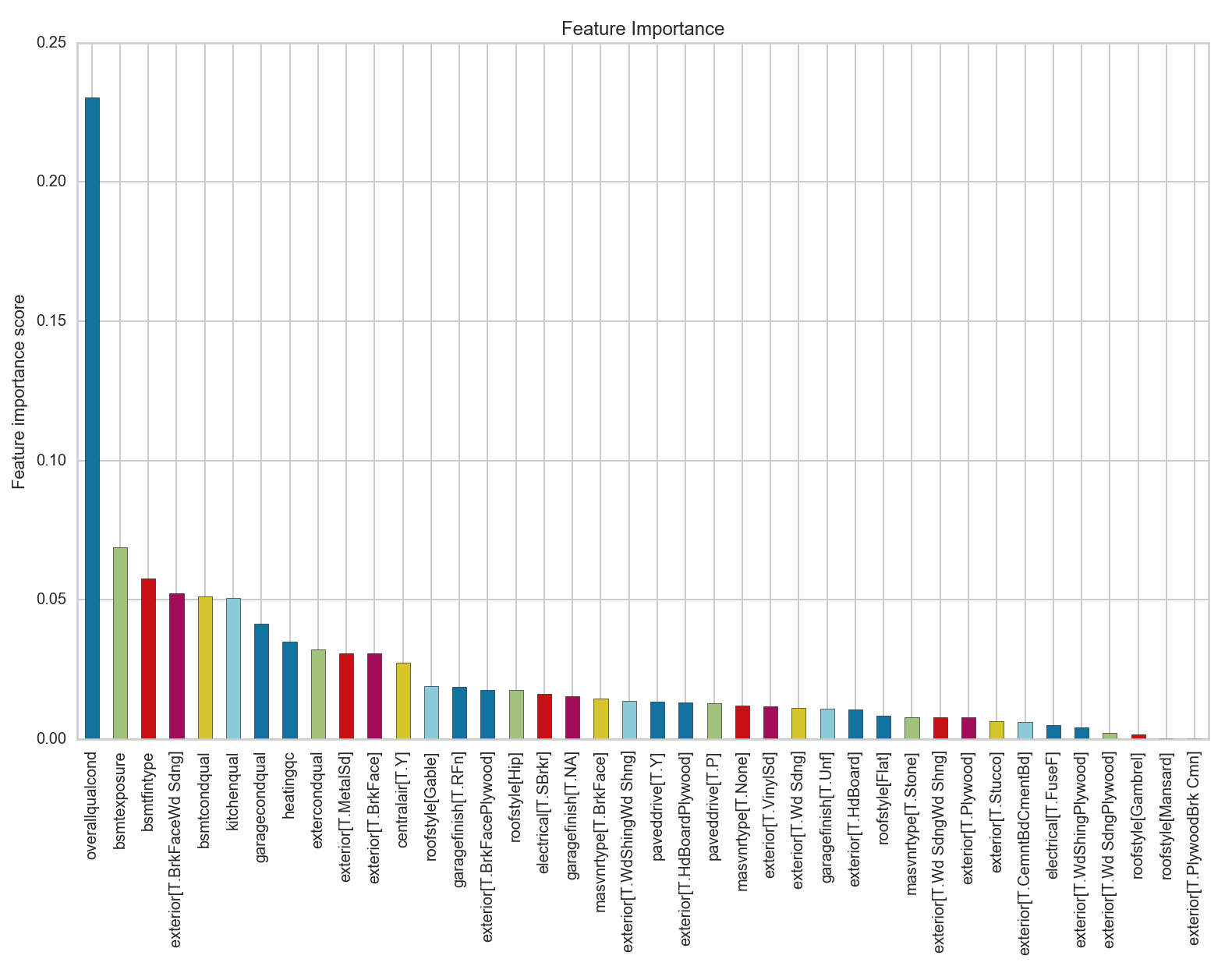
We see that the overall quality and condtion value of the house is more important than the next closest variable by a factor of 4. We will investigate this further by modeling all the features together instead of separating them into fixed and renovatable features.
Modeling with all features
We will model all preprocessed features and try to identify the impact our renovatable features have on our prediction accuracy.
We start with preparation of our X and y variables using Patsy
formula = 'saleprice ~ '+' + '.join([c for c in house.columns if not c == 'saleprice' if not c=='saletype' if not c=='salecondition']) + ' -1'
print formula
y, X = patsy.dmatrices(formula, data=house, return_type='dataframe')
y = y.values.ravel()

print X.shape, y.shape

saleprice ~ mssubclass + mszoning + lotfrontage + lotarea + lotshape + lotconfig + neighborhood + bldgtype + housestyle + roofstyle + masvnrtype + masvnrarea + foundation + bsmtexposure + bsmtunfsf + heatingqc + centralair + electrical + grlivarea + bedroomabvgr + kitchenqual + fireplaces + garagetype + garagefinish + garagearea + paveddrive + yrsold + garageage + furnishage + condition + exterior + bsmtfinsf + porch + bath + bsmtfintype + overallqualcond + extercondqual + garagecondqual + bsmtcondqual + mosold_sin + mosold_cos -1
(1448, 182) (1448,)
We have 182 features after performing one-hot encoding.
Next we split into our train and test sets.
X_test = X.loc[house['yrsold'] == 2010, :]
X_train = X.loc[house['yrsold'] != 2010,:]
y_test = y[house['yrsold'] == 2010]
y_train = y[house['yrsold'] != 2010]
We model with Linear Regression first as a baseline.
model(LinearRegression(), X_train, X_test, y_train, y_test, bar_plot=False)

Model Report:
RMSE:  3.3288202285e+16
R2:  -1.74301533309e+23
As expected, there are multiple collinear features present in our extended feature set.
We model with an untuned gradient boosted regressor first followed by a tuned one. As before, we will leave out the hypertuning steps.
model(gbr_base, X_train, X_test, y_train, y_test, bar_plot=False)

Model Report:
RMSE:  21757.2610489
Accuracy:  0.925538982099
Our base accuracy with all features before hyperparameter tuning is already better than the model with just the fixed features with R2at 0.9251.
gbr_best_all = GradientBoostingRegressor(max_depth=22, min_samples_split=24, min_samples_leaf = 3,max_features='sqrt', n_estimators=25600, subsample=0.85, learning_rate=0.001, random_state=123)

model(gbr_best_all, X_train, X_test, y_train, y_test)

Model Report:
RMSE:  19932.789609
R2:  0.937503357079
Our R2 looks to have improved by about 1.2 percentage points. Let’s take a look at the residuals.
Xs_train = ss.fit_transform(X_train)
Xs_test = ss.fit_transform(X_test)

visualizer = ResidualsPlot(gbr_best_all)
visualizer.fit(Xs_train, y_train)
visualizer.score(Xs_test, y_test)
visualizer.poof()
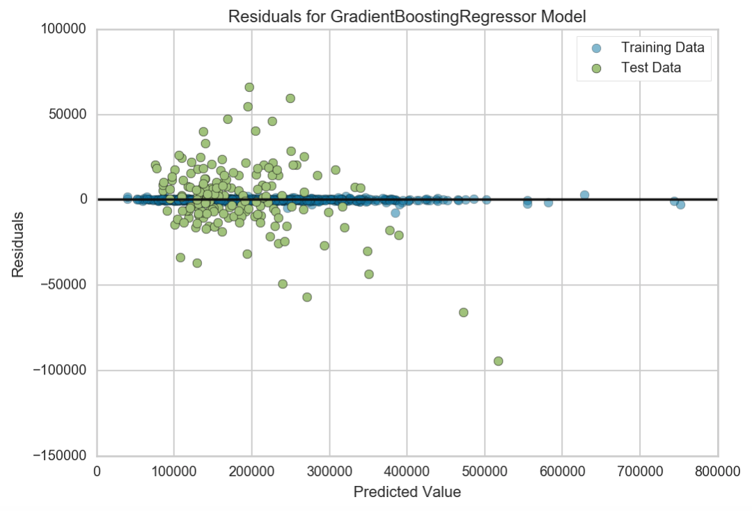
We can see that our training set has hardly any residuals, which suggests that this model with all the features accounts for almost all the variance in predicting the dependent variable. However, this is a clear sign of overfitting even though our R2 score on the test set seems to have improved.
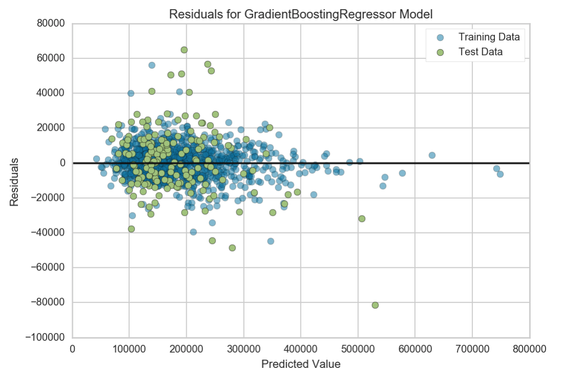
One interesting observation I had was when I fit the model with only the fixed features onto the full dataset with all features. The R2 score actually increased to 0.9431. The residual plot showed no clear pattern and the training set was not overfit.
model(gbr_best, X_train, X_test, y_train, y_test)

Model Report:
RMSE:  19011.1311829
R2:  0.943149218251
Hypothesis test for difference.
Let’s see if there’s a significant difference in this improvement in R2 values by performing a 2-sided T-test. Our null hypothesis states that there is no difference between the predicted values for the model with only the fixed features and the model with all features.
gbr_best.fit(Xs_train, y_train)
gbr_fixed = gbr_best.predict(Xs_test)

gbr_best_all.fit(Xs_train, y_train)
gbr_all = gbr_best_all.predict(Xs_test)

stats.ttest_ind(gbr_fixed, gbr_all)

Ttest_indResult(statistic=0.00447121767853376, pvalue=0.99643510323552464)
Our t-test result clearly shows that there is no difference between the predicted values using either model
Recommendations on type of houses to buy
Our results clearly show that the renovatable features of a house have very little impact on the property’s final saleprice, at least as can be observed from this dataset in Ames, Iowa. The low R2 score of 0.0565 suggests that renovatable features are unable to explain the differences seen in the predicted price with our fixed feature model and the actual saleprice of the houses very well.
This is further corroborated with the result of our hypothesis testing between the predicted values of both the fixed feature only model and the all feature model where there is no significant difference found in the values.
I would propose that a house be bought only when the predicted price with the gbr_best model (fixed features only) is at least $20,000 lower than the listed saleprice. This accounts for the RMSE amount seen in our best model of $19,011.
Summary
After extensive preprocessing and modeling, we were able to determine that renovatable features of the houses in Ames, Iowa do not matter as much as its fixed features in predicting saleprices. Our best model consisted only of fixed features and has an RMSE of $19,011.
The data was trained on pre 2010 data on 1276 observations and tested on 172 samples with transactions all occuring in 2010. While this model held true in 2010, it would be more prudent to continue updating the model with new data as we progress through the years. It might evolve to place more emphasis on renovatable features as markets and tastes change over time.